Portfolio / AI Learning Lab / Batch 02

Deep Learning · 2 study sheets

Batch 02

Follow the supplied sheets from neurons, losses, gradients, and CNNs to tokens and the transformer learning process.

One artificial neuron: inputs x1 and x2 weighted, summed with bias, passed through activation f

Deep Learning · sheet 1 of 2 in this chapter

Deep Learning and CNNs

Deep Learning Beginner → Intermediate structured sheet · Batch 2 math: no external renderer needed

1The neuron: weights, bias, activation

The question: what is a “neuron” doing, mechanically, when it receives numbers?

Intuition

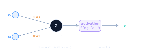
A neuron is a tiny weighted vote. Each input gets a say proportional to its weight, one adjustable bias sets the neuron’s eagerness to fire, and an activation function squashes the vote into a decision. Intelligence — such as it is — comes from stacking millions of these votes into layers and tuning all the weights.

One neuron: a weighted sum plus bias, passed through a nonlinear activation.

Technical

Weights (w) — learned multipliers; sign = excite/inhibit, magnitude = importance. This is what training updates.
Bias (b) — learned offset; lets the neuron fire even with all-zero input. Shifts the decision threshold.
Activation f — the nonlinearity. Without it, any stack of layers collapses algebraically into a single linear map: f(W₂·(W₁x)) = (W₂W₁)x — depth would buy nothing. Common choices: ReLU max(0, z) (default in CNNs), GELU (transformers), sigmoid/softmax (output layers).
Layer — a column of neurons that each see the same inputs. A dense layer with n inputs and m neurons = an n × m weight matrix + m biases.

Common misconception

“Neurons in a network are like biological neurons.” The analogy is loose at best: an artificial neuron is a multiply–add–nonlinearity unit; it has no spikes, timing, or neurotransmitters. The name is historical inspiration, not simulation.

Knowledge check

Why does removing every activation function collapse an 8-layer network into something a 1-layer network could express? Answer: composing linear maps yields a linear map (W₈···W₁ = W′). Only the interleaved nonlinearities make depth expressive.

2Forward propagation

The question: how does an input become a prediction, layer by layer?

Intuition

Each layer transforms its input into a slightly more abstract representation: pixels → edges → shapes → parts → objects. Forward propagation is just feeding numbers through this assembly line — no learning yet, just computation with the current weights.

Technical — one layer

z = Wx + b · a = f(z)

Stack L layers and feed each layer’s activations as the next layer’s inputs. Shapes: a batch of inputs (B, n₀) flows through (B, n₁) → … → (B, n_L).

Concrete example — one neuron by hand

Inputs x = [2, 1], weights w = [3, −1], bias b = 1, activation ReLU:

z = 3·2 + (−1)·1 + 1 = 6 → a = ReLU(6) = 6

If instead x = [2, −8]: z = 6 + 8 + 1 = 15 → a = 15; and with weights [−1, 1]: z = −2 −8 + 1 = −9 → ReLU(−9) = 0 — the neuron is silent. Negative z means “does not fire” under ReLU.

Knowledge check

A dense layer maps 784 → 128. How many parameters? Answer: 784 × 128 weights + 128 biases = 100,480. Parameters grow with input size — one motivation for weight sharing in CNNs (§7).

3Loss functions

The question: by what number do we judge a prediction “wrong”?

Intuition

The loss is the model’s single report-card number: low = predictions close to truth. Training is nothing more than the search for weights that make this number small. Choose the loss to match the task — the wrong loss optimizes for the wrong thing.

Technical

Regression — Mean Squared Error:

MSE = (1/n) Σ (y_i − ŷ_i)²

Classification — cross-entropy. If the model assigns probability p to the correct class:

L = −ln(p)

Confidently correct → p ≈ 1 → loss ≈ 0. Confidently wrong → p → 0 → loss → ∞. The logarithm punishes confident mistakes disproportionately, which keeps gradients informative.

Connect to our GPT: next-token prediction is classification over the vocabulary (65 classes for TinyShakespeare). That is why the untrained model’s loss is ln(65) ≈ 4.17 — the log of uniform probability 1/65 (see the Transformers sheet below, §9).

Common misconception

“Accuracy can be a loss function.” No — accuracy is a step function: a slightly-better prediction usually changes nothing, so it has zero gradient almost everywhere. We train on smooth surrogates (cross-entropy) and report accuracy.

Knowledge check

Model A assigns p = 0.6 to the truth; Model B assigns p = 0.05. Cross-entropy for each? Answer: −ln(0.6) ≈ 0.51; −ln(0.05) ≈ 3.00. B is ~6× worse — the log amplifies confident wrongness.

4Backpropagation & gradient descent

The question: with millions of weights, how does the network know which ones to blame for the error?

Intuition

Backpropagation is systematic blame assignment. The error is measured at the output, then the chain rule walks it backwards through every operation, asking each weight: “if I nudge you, how does the loss change?” Gradient descent then nudges every weight a tiny step in its own blame-reducing direction.

Gradient descent: w ← w − η · dL/dw. The slope shrinks near the minimum, so steps naturally get smaller. η (learning rate) scales every step.

Technical — the chain rule, in one worked example

Model: ŷ = w·x. Truth: y = 8. Input: x = 2. Current weight: w = 3. Loss: L = (ŷ − y)².

Forward: ŷ = 3 × 2 = 6 → L = (6 − 8)² = 4.
dL/dŷ = 2(ŷ − y) = 2(6 − 8) = −4.
dŷ/dw = x = 2.
Chain rule: dL/dw = (−4) × 2 = −8. Interpretation: increasing w decreases the loss strongly (negative gradient points downhill).
Update with η = 0.1: w ← 3 − 0.1×(−8) = 3.8.
Re-forward: ŷ = 7.6, L = 0.16. Loss fell 4 → 0.16 in one step.

Backpropagation is exactly this, applied to every weight of every layer simultaneously — the chain rule threaded through the whole computational graph, sharing intermediate results so the total cost is only ~2× the forward pass. No weight is “told” anything manually; every gradient is computed mechanically from the loss.

Cross-link: Transformers: From Tokens to Learning §9 shows this same loop at the GPT level (loss over 16,384 predictions → AdamW); here you’ve seen it at the single-weight level.

Common misconception

“Backpropagation is a learning algorithm.” It is only the gradient computation — efficient bookkeeping for the chain rule. The learning algorithm is gradient descent (or a variant, §5), which uses those gradients to update weights.

Knowledge check

In the worked example, if x had been 0, what gradient would w receive — and why is that a problem for training? Answer: dL/dw = 2(ŷ−y)·x = 0 regardless of the error. With zero input the weight is unblamed and unupdated; this is one root of vanishing-gradient and dead-neuron issues (e.g., ReLU units stuck below 0).

5Optimizers & learning rates

The question: raw gradient descent works — why does everyone use something fancier?

Intuition

Plain SGD is a drunkard walking downhill in the fog: honest direction, jerky pace. Momentum gives him a rolling ball (smooths zig-zag). Adam gives him adaptive footwear — a personalized step size per parameter based on the terrain history.

Technical

Optimizer	Update idea	Notes
SGD	w ← w − η·g	g = batch gradient. Simple, sometimes better final generalization, needs careful η.
SGD + momentum	velocity ← β·velocity + g; w ← w − η·velocity	Averages recent gradients; accelerates consistent directions, damps oscillation.
Adam	per-parameter scaling by running mean & variance of g	Robust default; works with little tuning. AdamW = Adam with decoupled weight decay — the correct regularization form.

Learning rate — the hyperparameter that matters most:

Too large → loss oscillates or explodes (NaNs).
Too small → glacial progress, risk of getting stuck.
Schedules — warmup (ramp from ~0 over the first ~100 steps: early gradients are wild) then decay (cosine or step-down: fine adjustments need fine steps).
Connect to our GPT: train.py uses AdamW, betas (0.9, 0.95), grad clipping at 1.0, and a 100-step linear warmup into cosine decay — every element of this section, live.

Common misconception

“Adam is always better than SGD.” Adam is the safer default, but SGD+momentum still wins some vision benchmarks at full training budgets. Also, Adam’s per-parameter step sizes reduce the meaning of η comparisons across optimizers — always re-tune η when switching.

Knowledge check

Your loss spikes to NaN mid-training. Name the first three knobs to check. Answer: (1) learning rate too high; (2) no/low gradient clipping (our code clips at 1.0); (3) warmup missing or too short — early-training explosions are common. (Numerical instability under mixed precision is a fourth candidate.)

6Epochs, batches, iterations

The question: “the model trained for 5000 steps” — how much data is that?

Technical — the three words

Batch (iteration) — one forward + backward + update pass on B examples.
Epoch — one full pass over the training set: iterations/epoch = ⌈N / batch_size⌉.
Step — usually synonymous with iteration (some papers count optimizer steps under gradient accumulation differently).

Example: N = 10,000, batch 64 → 157 iterations per epoch; 20 epochs = 3,140 iterations.

Cross-link: the GPT Training Data Flow sketch (standalone file in the Lab) is entirely about this — including why our GPT loop (5000 random batches over a 1.1M-token stream) has no fixed epoch: batches are sampled with replacement, so a step count never guarantees full coverage. Batch size in that repo = 64 sequences × 256 tokens = 16,384 tokens per step — quantified again in the Transformers sheet §9 below.

Knowledge check

Why does a larger batch often allow a larger learning rate? Answer: averaging over more examples reduces gradient noise (variance ∝ 1/B), so bigger steps stay stable — the basis of linear-scaling rules of thumb. Trade-off: large batches reduce per-epoch update count and may generalize slightly worse at fixed compute.

7Convolution: kernels, feature maps, stride, padding

The question: why don’t CNNs just flatten the image into a dense layer?

Intuition

A 1000×1000 RGB image flattened is 3 million inputs; a dense layer with 1000 neurons = 3 billion parameters, and it would have to relearn “an edge is an edge” for every pixel position. A convolution instead slides one tiny pattern-detector (kernel) across the whole image: the same edge detector, applied everywhere. Weight sharing + local connectivity.

Technical — the operation

Place the K×K kernel over a patch of the input; multiply element-wise; sum; write one output number. Slide by stride S. Padding P zeroes a border to control output size. One kernel produces one feature map (channel); a conv layer applies F independent kernels, giving F feature maps.

output size = ⌊(N − K + 2P) / S⌋ + 1

Parameters per layer: F × (K × K × C_in) + F — independent of image size!

One convolution output, computed by hand. With 16 kernels you get 16 such maps — each a different learned pattern applied at every position.

Stride & padding effects

N	K	P	S	Output	Meaning
5	3	0	1	3	figure above — no padding
5	3	1	1	5	“same” padding — size preserved
32	3	1	1	32	typical modern conv (our §9 walkthrough)
5	3	0	2	2	stride 2 downsamples (~like pooling)

Common misconception

“Convolution flips the kernel” — the strict mathematical definition does; deep-learning implementations skip the flip (they compute cross-correlation). Since the kernel is learned, the distinction has zero practical effect.

Knowledge check

Input 224×224×3, 64 kernels of 7×7, stride 2, padding 3. Output size and parameter count? Answer: size ⌊(224 − 7 + 6)/2⌋ + 1 = 112 → (112, 112, 64). Params = 64×(7·7·3) + 64 = 9,472 — independent of the 224. (This is the stem of ResNet-style networks.)

8Pooling & receptive fields

The question: after detecting features, how does the network become tolerant to small shifts — and see bigger context?

Intuition

Max pooling asks each 2×2 neighborhood: “did the feature appear here at all?” — keeping the strongest response and discarding the exact position. That buys translation tolerance, shrinks the map, and (critically) makes each deeper neuron look at a wider slice of the original image.

Technical

Max pool 2×2, stride 2 — halves H and W; no learnable parameters; per-channel.
Average pooling — smoother; global average pooling (GAP) collapses each final map to a single number, replacing big flatten+FC heads.
Receptive field — the input region influencing one output neuron. With two stacked 3×3 convs: the second layer sees 5×5 of the input; add a 2×2 pool and the next conv spans more. Deep stacks trade resolution for semantic reach — exactly what classification needs.

Common misconception

“Pooling is what extracts features.” No — convolutions detect; pooling only summarizes and downsamples. Modern architectures sometimes replace it with strided convs (learnable downsampling).

Knowledge check

Why does max pooling have no parameters and no real “training”? Answer: max is a fixed selection rule — there is nothing to learn. Its inductive bias (local invariance) is hard-coded; gradients simply pass through to the arg-max input (and zeros elsewhere).

9A CNN end to end — every tensor shape traced

The question: what actually happens to a 28×28 image on its way to “this is a 7”?

The canonical rhythm: conv → nonlinearity → pool, repeated, then flatten and a classifier head. Spatial size shrinks, channel count grows, until the classifier works on “concepts” rather than pixels.

Why the shapes work out

Pad-1 convs preserve 28→28 and 14→14; pools do all the shrinking (÷2 each time).
Channel count doubles (1→16→32) as spatial size halves — the standard budget shift.
Flatten turns the final (32, 7, 7) volume into a 1,568-vector; the linear head maps it to 10 class logits; cross-entropy + argmax finish the job.
Modern refinements: BatchNorm after each conv (stabilizes activations), ResNet skip connections out = f(x) + x (lets 50–150-layer nets train — He et al., 2015), GAP heads instead of big FC layers.

Knowledge check

Without the two pools, what would the flatten size be, and why might training be worse? Answer: (32, 28, 28) → 25,088 features: a 16× bigger head (≈400K params instead of 15.7K) that overfits easily, with less translation tolerance built in along the way.

10Transfer learning & fine-tuning

The question: you have 800 labeled images. Why train from scratch is the wrong move?

Intuition

A network pretrained on ImageNet already knows edges, textures, parts, and object-ness — the first ~80% of your problem. You harvest that knowledge and only re-learn the last mile: your categories. Less data needed, faster, and usually more accurate.

Technical — the two modes

Mode	What moves	When
Feature extraction	Backbone frozen; train only the new head	Small dataset, similar to pretraining domain
Fine-tuning	Unfreeze top block (often deeper layers only) with a low LR	Larger dataset, or noticeably different domain (medical scans, satellite)

Why a low LR when fine-tuning? Pretrained weights sit in a good basin; big steps destroy them. Typical recipe: head at 1e-3, backbone at 1e-5 (discriminative LRs).

Connect forward: this is precisely the bridge to LLM fine-tuning — LoRA/QLoRA (your GPT Phase 2) is parameter-efficient fine-tuning applied to language models instead of CNN backbones.

Common misconception

“Fine-tuning always beats feature extraction.” With a small dataset, unfreezing the backbone just adds overfitting surface. Choose by (data size × domain distance), not by fashion.

Knowledge check

Task: classify X-ray fractures; you have 600 images. Which mode, and which LR discipline? Answer: start with feature extraction (frozen backbone, new head); if validation underfits, unfreeze the top block only, LR ≈ 1e-5 for the backbone — domain is far from natural images, so some backbone adaptation helps, but data is too scarce to retrain it all.

11Data augmentation & regularization in DL

The question: the CNN overfits — what are the vision-specific levers?

Technical

Augmentation — random flips, crops, rotations, color jitter, Cutout/MixUp: label-preserving distortions that multiply effective data. Rule: the transform must not change the label (a flipped “6” is not a “9”; digit recognition must skip horizontal flips).
Dropout — randomly zero activations in FC heads (typically p = 0.2–0.5).
Weight decay — L2 penalty via AdamW.
Early stopping — keep the checkpoint at the validation minimum.
BatchNorm — normalizes layer inputs over the batch; stabilizes and mildly regularizes. (Contrast with the LayerNorm used in transformers — per-token, batch-independent — the Transformers sheet §6 below.)

Cross-link: the bias–variance diagnosis table and the train/val curve logic live in Machine Learning Fundamentals §4–5 (your Stage 1 file) — same disease, deep-learning-specific medicine here.

Knowledge check

Why does augmentation act as a regularizer rather than “more information”? Answer: it encodes an invariance prior — the model is rewarded for predicting the same label under nuisance transforms, so it spends capacity on invariant, transferable features instead of memorizing incidental details.

12Quiz

Attempt each before expanding.

Q1 — A 3×3 conv on a 16-channel input with 32 filters: parameter count?

32 × (3·3·16) + 32 = 4,640. The +32 is one bias per filter. Note it does not depend on the input H×W — that is weight sharing. (§7)

Q2 — N=32, K=5, P=2, S=1: output size? What is this padding recipe called?

⌊(32 − 5 + 4)/1⌋ + 1 = 32 — “same” padding: K odd, P = (K−1)/2 preserves size. (§7)

Q3 — Stack of linears without activations: what function class, and what does that imply for depth?

A single linear map (matrix product). Depth adds nothing without interleaved nonlinearities. (§1)

Q4 — In our GPT, 5000 iterations with batch 64×256 tokens over 1.1M tokens: roughly how many “epochs”, and why is the number ill-defined?

≈ 5000·16,384 / 1.1M ≈ 74 passes worth of tokens — but batches are sampled with replacement, so coverage is uneven and no true epoch counter exists. (§6)

Q5 — 600 labeled X-rays: feature extraction or fine-tuning, and why?

Feature extraction first (tiny dataset — a trainable backbone would overfit); optionally unfreeze the top block at ~1e-5 if validation shows underfitting. (§10)

Q6 — Your training loss is stuck at 2.3 and oscillating wildly. Three suspects?

Learning rate too high; warmup missing; no gradient clipping. (BatchNorm absent / bad init are follow-ups.) (§5)

13Exercise — conv2d forward, from scratch

Implementation challenge

Implement single-channel 2D convolution (stride 1, padding 0) in NumPy, verify it against the §7 hand example, then check shapes against PyTorch. Stretch: add stride/padding, then im2col.

# conv_exercise.py — pip install numpy torch
import numpy as np

def conv2d(x, k):
    """x: (H, W), k: (K, K) → out: (H-K+1, W-K+1), stride 1, pad 0."""
    H, W = x.shape; K = k.shape[0]
    Ho, Wo = H - K + 1, W - K + 1
    out = np.zeros((Ho, Wo))
    for i in range(Ho):
        for j in range(Wo):
            out[i, j] = np.sum(x[i:i+K, j:j+K] * k)   # multiply-overlay-sum
    return out

x = np.array([[1,2,3,2,1],
              [4,5,6,3,2],
              [7,8,9,4,3],
              [5,4,3,2,1],
              [2,3,4,5,4]])
k = np.array([[0,1,0],
              [1,4,1],
              [0,1,0]])
out = conv2d(x, k)
assert out.shape == (3, 3)
assert out[0, 0] == 40, out   # must match the hand computation in §7
print(out)

# Cross-check with PyTorch (1 input channel, 1 filter):
import torch, torch.nn.functional as F
t = F.conv2d(torch.tensor(x).float()[None, None],
             torch.tensor(k).float()[None, None])
assert np.allclose(out, t[0, 0].numpy())

Deliverables: (1) all asserts pass; (2) one-paragraph answer: why is the nested-loop version slow, and how does im2col turn conv into one matrix multiply? Stretch: generalize to stride s and padding p and re-verify against F.conv2d(..., stride, padding); then run your §9 CNN in PyTorch and print every shape.

14References

CS231n — Convolutional Networks for Visual Recognition (Stanford), course notes: cs231n.github.io/convolutional-networks
Goodfellow, Bengio, Courville — Deep Learning, ch. 6 (MLPs) & ch. 9 (CNNs): deeplearningbook.org
He et al. — “Deep Residual Learning for Image Recognition” (ResNet), arXiv:1512.03385: arxiv.org/abs/1512.03385
Krizhevsky, Sutskever, Hinton — “ImageNet Classification with Deep CNNs” (AlexNet), NeurIPS 2012: papers.nips.cc
PyTorch — torch.nn.Conv2d documentation: pytorch.org/docs
Kingma & Ba — “Adam: A Method for Stochastic Optimization,” arXiv:1412.6980: arxiv.org/abs/1412.6980

Primary or official sources, links verified at writing time. Identify any simplification you rely on; when in doubt, check the paper.

Progress checklist

Ticks persist in this browser only (localStorage).

I can compute a neuron’s output by hand and explain why activations are necessary.
I reproduced the w = 3 → 3.8 backprop example without looking.
I can name when to use AdamW vs SGD+momentum and read a warmup+cosine schedule.
I can compute conv output size and parameter count from N, K, P, S, F, C_in.
I can trace the (1,28,28) → … → 10 walkthrough and justify every shape.
I can choose between feature extraction and fine-tuning given data size and domain distance.
Exercise done: conv2d matches PyTorch.

Provenance: structured sheet from Batch 2 of the AI Learning Lab project — a personal study resource, not a claim of expertise. Verify specifics against the references before use in graded work.

Last reviewed: not yet — set this date after your first full pass.

Transformers and LLMs · sheet 2 of 2 in this chapter

Transformers: From Tokens to Learning

Transformers and LLMs Intermediate structured sheet · Batch 2 companion to the sketch sheets (standalone files)

0How this sheet relates to the Lab

This is the mechanics sheet for the Transformer story. Two sketch sheets in the Lab (“How a Transformer Learns and Generates”, “GPT Training Data Flow”) give the mental movies as standalone files; Stage 1 gave you the evaluation discipline. This sheet gives you the numbers — nothing here re-argues the big picture, it zooms in.

Topic	Where you met it	This sheet (mechanics)
The weight-level learning loop	Deep Learning and CNNs §4 (single weight)	§9–11 here — the same loop at sequence scale
Batching & tokens per step	GPT Training Data Flow sketch (standalone)	§9 — where the targets come from (y = x shifted)
Attention (which token looks where)	Transformer sketch (standalone)	§3–5 — one head computed by hand, then multi-head
Code	—	every section maps to a named piece of `model.py` from our GPT repo

1From text to token IDs

The question: the model only does matrix math — how does text become numbers?

Intuition

A tokenizer is the model’s dictionary: it chops text into standard pieces (tokens) and looks up each piece’s ID in a fixed vocabulary. “unbelievable” might become un + believ + able — three IDs the model has seen thousands of times, rather than one word it has never seen at all.

Technical

Character-level — vocab = every distinct character (TinyShakespeare: 65). Simple, but sequences get long and every token carries little meaning.
BPE (byte-pair encoding) — start from 256 bytes; repeatedly merge the most frequent adjacent pair into a new token. GPT-family models use BPE variants; vocabularies run ~50K–200K. Our repo ships both: tokenizer.py (char) and the BPE you built against a pytest spec.
The vocabulary is fixed before training — the model never learns new tokens, only what the existing ones mean.

Connect to model.py: tok_emb = nn.Embedding(vocab_size, n_embd) — row id of that matrix is the token’s learned vector.

Common misconception

“The model sees words or letters.” It sees neither — it sees IDs over an arbitrary subword vocabulary. This explains oddities like models miscounting letters in “strawberry”: the tokenizer may not even present the letters separately.

Knowledge check

Why can BPE represent any text, even gibberish like “zzzqqq”, with a 500-token vocab? Answer: BPE is built on the 256 raw bytes as a fallback — any byte sequence is encodable; frequent sequences just get shorter representations. Round-trip decode(encode(x)) == x always holds.

2Embeddings & positional information

The question: why does the input to block 1 have an extra “position” part added?

Intuition

The embedding lookup turns each token ID into a learned vector — its “meaning so far.” But attention has no built-in sense of order: shuffle the input tokens and attention alone produces the shuffled output. So we inject position explicitly: one vector for what, one for where.

Technical

x₀ = Embedding_tok(id) + Embedding_pos(position)

Learned absolute positions (GPT-2, our model.py) — a block_size × n_embd table; position 300 simply doesn’t exist if block_size = 256. This is why generate() crops the context.
Sinusoidal (original Transformer) — fixed geometric pattern; extrapolates a bit beyond trained lengths.
RoPE (modern LLMs — Llama, Qwen) — rotates Q/K pairs by position-dependent angles, so relative distance appears in the attention score; the basis of modern long-context tricks. Simplification: RoPE is applied inside attention, not added at input — details in the RoPE paper.

Common misconception

“Positional embeddings tell the model grammar.” They only stamp order. Everything the model does with that order (syntax, long-range coherence) is learned in the blocks.

Knowledge check

You zero out pos_emb at inference (experiment #7 from the repo). What degrades — word identity or word order? Answer: word order. Token identity is intact (token embeddings remain); the model can no longer distinguish “dog bites man” from “man bites dog.”

3Query, Key, Value

The question: how does one token decide which other tokens matter to it?

Intuition

Think of a soft database lookup. Every token advertises a Key (“here’s what I contain”) and holds a Value (“here’s what I can hand you”). The current token issues a Query (“here’s what I’m looking for”). Compare the query to every key; the better the match, the more of that token’s value flows into you.

Technical

All three are learned linear projections of the same input x — three weight matrices updated by backprop:

Q = x·W_Q K = x·W_K V = x·W_V

In model.py these are one fused nn.Linear(n_embd, 3·n_embd) split into three — mathematically identical, faster on GPU. The retrieval analogy is soft: Q·K is content-based addressing with graded, differentiable matches — not exact key lookup.

Knowledge check

Which of Q, K, V does a token use to receive information, and which to send? Answer: receives via its Q (matched against others’ K); sends via its V (weighted by how well its K matches others’ Q). K and V can differ: what makes a good “label” isn’t what makes good “content.”

4Scaled dot-product attention — worked by hand

The question: what does each operation in Attention(Q,K,V) actually compute?

The formula

Attention(Q, K, V) = softmax( Q·K^T / √d_k ) · V

Worked example — d_k = 4, one query, two candidate keys

q = [1, 0, 1, 0] · k₁ = [1, 0, 1, 0] · k₂ = [0, 1, 0, 1]
v₁ = [1, 2, 3, 4] · v₂ = [10, 20, 30, 40]

Dot products (compatibility): q·k₁ = 1+1 = 2; q·k₂ = 0. The query matches k₁ strongly, k₂ not at all.
Scale by √d_k = 2: scores become 1.0 and 0. Why scale? For large d_k, dot products of random vectors have variance ∝ d_k; unscaled, softmax saturates into near-one-hot gradients-dead outputs. Dividing by √d_k normalizes the variance and keeps softmax in its responsive region.
Softmax: e^1.0 ≈ 2.718; e⁰ = 1; sum ≈ 3.718 → weights 0.731 and 0.269 (they sum to 1 — attention is a mixture, not a selection).
Weighted sum of values: 0.731·[1,2,3,4] + 0.269·[10,20,30,40] = [3.42, 6.84, 10.26, 13.68].

Read the output: it is mostly v₁, tinted by v₂. In a real block there are T such queries — one output vector per token — computed for the whole sequence in one matrix multiply. That parallelism is a large part of why transformers displaced RNNs.

Common misconception

“Attention picks the most relevant token.” It doesn’t select — it averages, with learned weights. Even a 0.05-weight token contributes. (Hard selection appears only via sampling at generation time, which is a different mechanism entirely.)

Knowledge check

In step 3, why must the weights sum to exactly 1? Answer: softmax normalizes the scores into a probability distribution. The output is then a convex combination of value vectors — bounded, stable, and interpretable as “how much attention came from where.”

5Multi-head attention

The question: one attention pattern per layer seems poor — how do several help?

Intuition

One head can track one relation type at a time: maybe “who is the subject?” But a token may need to watch a pronoun’s antecedent, the current verb, and the punctuation rhythm simultaneously. Give the layer several small attentions in parallel — heads — each free to learn its own Q/K/V and its own pattern.

Technical

Split d_model across h heads: each head works in d_head = d_model/h dimensions, runs the §4 pipeline independently, then all head outputs are concatenated and mixed by a final projection W_O:

MHA(x) = Concat(head₁,…,head_h)·W_O

Our GPT: n_embd = 384, n_head = 6 → head_dim = 64. Same total computation as one 384-dim attention, but six specialized subspaces instead of one. Simplification: heads are not guaranteed to be cleanly interpretable; “each head learns one linguistic rule” is an idealized story that only sometimes holds in practice.

Multi-head: same parameter budget as one big attention, but several relation types can be tracked in parallel.

Knowledge check

If n_embd = 512 and n_head = 8, what is head_dim, and why does concatenating eight 64-dim outputs restore the original width? Answer: 512/8 = 64; concat of 8 × 64 = 512, then W_O (512×512) mixes across heads. Total attention params stay O(d²), not O(h·d²).

6The rest of the block: FFN, residuals, LayerNorm

The question: attention moves information between tokens — who processes it once it arrives?

Technical — the three remaining parts

FFN / MLP — per-token, position-wise: expand 4× (384 → 1536 in our GPT), GELU, project back. This is where most parameters live (~2/3 of the block) and where much “knowledge” is stored. Attention = communicate; MLP = compute.
Residual connections — x = x + attn(ln x), x = x + mlp(ln x) (pre-norm, as in GPT-2 and our model.py). The addition creates a gradient highway: during backprop, gradients flow through the + unchanged, letting deep stacks train. Also: each block only has to learn an increment on the representation.
LayerNorm — normalizes each token’s vector across its features (mean ≈ 0, unit-ish variance, learned scale/shift). Keeps activation scales stable across depth. Placed before each sublayer (pre-norm). Contrast: BatchNorm normalizes across the batch — awkward for variable-length sequences, which is why transformers use LN.

Common misconception

“Residual connections are an optimization trick only.” They help optimization, yes — but they also change the function class: the network learns residual refinements stacked on a running representation, which is part of why 100+ layer transformers are trainable at all.

Knowledge check

Why is pre-norm (x + f(ln x)) preferred over post-norm (ln(x + f(x))) in deep GPT-style stacks? Answer: pre-norm keeps a clean identity path from bottom to top — gradients reach layer 1 undiminished. Post-norm’s path passes through a normalization at every block, which historically needed careful warmup to train at depth.

7Three architecture families

The question: BERT, GPT, T5 — all “transformers.” What actually differs?

Technical — one axis: the attention pattern

Same blocks, different wiring. The attention pattern is the identity of the family.

Encoder-only — bidirectional attention; trained with masked-token / contrastive objectives; outputs representations, not text. (BERT, embedding models — including RAG retrievers!)
Decoder-only — causal attention; trained on next-token prediction; generates. (GPT, Llama, Qwen — and everything in your roadmap.) Dominant because one objective scales endlessly.
Encoder–decoder — encoder understands, decoder generates with cross-attention into encoder states. (T5, BART; original Transformer was this form for translation.)

Knowledge check

Your RAG embedding model (all-MiniLM) is which family, and why does that family suit retrieval? Answer: encoder-only — bidirectional attention means the sentence representation incorporates context from both sides; you need a good fixed vector per text, not generation.

8Causal masking

The question: training predicts all positions at once — what stops token 3 from reading token 4’s answer?

Technical

A lower-triangular matrix of allowed positions is added to the attention scores before softmax: future positions get −∞, so softmax assigns them exactly 0. In model.py: torch.tril(...), registered as a buffer, sliced to the current T each forward.

Row = who is looking; column = what is looked at. Future = masked. Row sums stay 1 after softmax (e.g., row w₃ redistributes over {w₁, w₂, w₃}).

Why this is clever

Thanks to the mask, one training pass yields T supervised predictions in parallel — position 1 predicts from {w₁}, position 2 from {w₁,w₂}, and so on. No RNN-style sequential unrolling, no peeking. Same trick at inference: generate() crops the context to the last block_size tokens and every position still attends only leftward.

Knowledge check

You accidentally disable the mask during training, then fix it at inference. What does the model have (and not have) that breaks generation? Answer: it learned distributions that depend on future tokens — a habit it cannot use at inference, since the future doesn’t exist yet. Its next-token outputs are meaningless in exactly the cases (mid-sequence positions) that training optimized.

9Next-token prediction & the loss

The question: where do the “labels” for a language model come from?

Technical — targets are the input, shifted

In data.py: x = stream[i:i+T], y = stream[i+1:i+T+1]. Position t of x must predict the token at position t of y. The model’s head produces logits (one raw score per vocab entry); cross-entropy with the true next token gives the loss; −ln p is the same formula as the CNN sheet §3, just over 65 (or 50K) classes.

The famous sanity check: an untrained model outputs ≈uniform logits → p(correct) ≈ 1/65 → loss = ln(65) ≈ 4.17. Our train.py prints this before training begins. Watch loss go 4.17 → ~1.5: that’s the model moving from uniform guessing to confidently right — in a loss sense; decoding behavior is §11.

Common misconception

“Loss 1.5 means the model is 1.5 confused” or “accuracy = 1 − loss/…” — no. Loss is −ln p of the correct token, averaged. It has no direct percent interpretation; compare only across identical tokenization and data. (Recall from the BPE milestone: switching tokenizers changes the scale — bytes/token and sample quality are the honest comparison.)

Knowledge check

A batch has B=64, T=256. How many next-token predictions contribute to one loss value? Answer: B × T = 16,384 — every position of every sequence is a supervised example. This dense supervision is why 5,000 steps suffice to see clear learning on 1.1M tokens.

10Training vs inference

The question: same forward pass — what exactly differs?

Technical — a precise diff

Aspect	Training	Inference
Inputs	x and targets y (shifted stream)	prompt only; targets are the model’s own outputs
Loss / backward	cross-entropy → backprop → grads	none — forward pass only
Weights	updated by optimizer (AdamW)	frozen — nothing writes to them
Dropout	active (regularization)	off (deterministic network)
Sequence length	fixed windows of block_size	grows by 1 token per loop iteration (cropped to block_size)
Sampling	—	temperature / top-k over the final distribution

The activations inside the network change with every input in both modes; what never changes at inference is the parameter set. That distinction — activations vs parameters — resolves the classic beginner confusion “but the model computes different things, so isn’t it learning?”

Knowledge check

A friend says “ChatGPT learned from our conversation just now.” Correct this precisely. Answer: the conversation changed only the context fed to frozen weights (plus any provider-side retrieval/memory features, which are not weight updates). The model’s parameters are identical to before the chat.

11Autoregressive generation

The question: the model outputs a whole distribution — how does text actually appear?

Technical — the loop in `generate()`

The loop your generate() implements: predict → sample → append → repeat.

Temperature divides logits before softmax: <1 sharpens toward greedy, >1 flattens toward uniform; 0 (=argmax) is deterministic but repetitive.
Top-k keeps only the k highest-probability tokens before sampling — kills the long low-quality tail. (Top-p/nucleus: keep smallest set with cumulative mass ≥ p.)
Each iteration runs a full forward pass over the cropped context — correct, simple, O(T²) total for T tokens. (Production serving adds a KV cache to reuse past computations; that’s an engineering optimization, not a change to the math — see LLM Fundamentals, Stage 3, §10.)

Trace with our sampler

Prompt "ROMEO:", temperature 0.8, top_k 200 → logits/0.8 → mask all but top 200 → softmax → multinomial sample → append → repeat. High-probability continuations (a character name) dominate; occasionally a surprise word — that variance is the poetry. Set temperature 0.1 and the same checkpoint turns mechanical; 1.5 and it raves (repo experiment #6).

Common misconception

“The model plans the whole sentence, then types it.” No — each token is chosen from a distribution conditioned only on what came before. Long-range coherence emerges from extremely good next-token distributions, not from a stored plan.

Knowledge check

Why does generation slow down as the sequence grows (even before batch effects)? Two reasons? Answer: (1) the forward pass re-processes the entire (growing) context each iteration; (2) attention cost per pass grows with context length. KV caching removes most recomputation but per-token cost still grows with context.

12Quiz

Attempt each before expanding.

Q1 — Why divide Q·Kᵀ by √d_k? What breaks without it?

Variance of dot products grows with d_k → softmax saturates to near one-hot → gradients vanish. Scaling keeps scores in softmax’s responsive range. (§4)

Q2 — n_embd 384, 6 heads: head_dim? After concat and W_O, output width?

64; concat gives 384; W_O (384×384) mixes across heads → output stays 384. (§5)

Q3 — What loss value do you expect before training on a 50,000-token BPE vocab, and why?

≈ ln(50,000) ≈ 10.8 — uniform prediction over 50K classes. Same sanity-check logic as ln(65) ≈ 4.17 for char-level. (§9)

Q4 — Remove positional embeddings from a decoder-only model: what exactly fails?

Attention becomes permutation-agnostic — “dog bites man” and “man bites dog” become the same computation; word order information is simply absent. Token identity still works. (§2)

Q5 — Three differences between training and inference forward passes.

Targets present vs absent; backward/optimizer on vs off; dropout on vs off. (Also: fixed window vs growing context; no sampling during training.) (§10)

Q6 — Your roadmap’s first papers (Transformer → GPT-2 → …): which family do they belong to, and which single mechanism distinguishes it from BERT?

Decoder-only; causal (leftward-only) attention vs BERT’s bidirectional attention. (§7–8)

13Exercise — attention by hand, then in NumPy

Implementation challenge

Part A: verify the §4 numbers by hand (no code). Part B: implement masked scaled dot-product attention in NumPy and test it against the §4 vectors and against PyTorch.

# attn_exercise.py — pip install numpy torch
import numpy as np

def attention(Q, K, V, mask=None):
    """Q,K,V: (T, d). mask: (T, T) bool, True = allowed. Returns (T, d)."""
    d = Q.shape[-1]
    scores = Q @ K.T / np.sqrt(d)            # (T, T)
    if mask is not None:
        scores = np.where(mask, scores, -np.inf)
    scores -= scores.max(axis=-1, keepdims=True)  # numerical stability
    w = np.exp(scores); w /= w.sum(axis=-1, keepdims=True)
    assert np.allclose(w.sum(axis=-1), 1)     # rows are distributions
    return w @ V, w

# --- Test 1: the §4 hand example (d=4, two keys) --------------------------
q  = np.array([[1,0,1,0]])
K  = np.array([[1,0,1,0],[0,1,0,1]])
V  = np.array([[1,2,3,4],[10,20,30,40]])
out, w = attention(q, K, V)
assert np.allclose(w, [0.7311, 0.2689], atol=1e-3), w
assert np.allclose(out, [[3.42, 6.84, 10.26, 13.68]], atol=1e-2), out

# --- Test 2: causal mask + PyTorch cross-check ----------------------------
import torch, torch.nn.functional as F
T, d = 4, 8
rng = np.random.default_rng(0)
Q2, K2, V2 = (rng.normal(size=(T, d)) for _ in range(3))
mask = np.tril(np.ones((T, T), dtype=bool))
out2, w2 = attention(Q2, K2, V2, mask)
ref = F.scaled_dot_product_attention(
    torch.tensor(Q2)[None], torch.tensor(K2)[None], torch.tensor(V2)[None],
    is_causal=True)
assert np.allclose(out2, ref[0].numpy(), atol=1e-5)

Deliverables: (1) hand-verified §4 values; (2) both asserts pass — note the row-sums-to-1 assertion caught inside attention(); (3) stretch: wrap your attention in the 6-head split/concat from §5 and verify equality with a single-head call on reshaped tensors where all heads share weights (then explain in one paragraph why equality holds there and not in a real multi-head layer).

14References

Vaswani et al. — “Attention Is All You Need,” arXiv:1706.03762 (the Transformer, 2017): arxiv.org/abs/1706.03762
Radford et al. — “Language Models are Unsupervised Multitask Learners” (GPT-2, 2019): OpenAI (PDF)
J. Alammar — “The Illustrated Transformer”: jalammar.github.io
Harvard NLP — “The Annotated Transformer” (line-by-line implementation): nlp.seas.harvard.edu
Karpathy — nanoGPT: github.com/karpathy/nanoGPT · minbpe: github.com/karpathy/minbpe
Ba, Kiros, Hinton — “Layer Normalization,” arXiv:1607.06450: arxiv.org/abs/1607.06450
Su et al. — “RoFormer: Enhanced Transformer with RoPE,” arXiv:2104.09864: arxiv.org/abs/2104.09864

Primary papers and stable educational sources; verified at writing time. Where this sheet simplifies (heads interpretability, RoPE placement), the simplification is labeled in place.

Progress checklist

Ticks persist in this browser only (localStorage).

I can explain char-level vs BPE and why round-trip always holds.
I can state why positional information is needed and name three schemes.
I reproduced the d=4 attention example by hand (0.731/0.269, output [3.42, 6.84, 10.26, 13.68]).
I can compute head_dim and explain concat + W_O.
I can draw the pre-norm block from memory and say what residuals do for gradients.
I can classify BERT / GPT / T5 by attention pattern.
I can explain what the causal mask does and why training without it ruins generation.
I can predict initial loss ln(V) for any vocab size.
Exercise done: NumPy attention matches PyTorch with is_causal=True.

Last reviewed: not yet — set this date after your first full pass.

The source material is preserved in full. Open the complete original HTML collection.

Batch 02

Deep Learning, CNNs & Transformer Mechanics

1The neuron: weights, bias, activation

Intuition

Technical

Common misconception

2Forward propagation

Intuition

Technical — one layer

Concrete example — one neuron by hand

3Loss functions

Intuition

Technical

Common misconception

4Backpropagation & gradient descent

Intuition

Technical — the chain rule, in one worked example

Common misconception

5Optimizers & learning rates

Intuition

Technical

Common misconception

6Epochs, batches, iterations

Technical — the three words

7Convolution: kernels, feature maps, stride, padding

Intuition

Technical — the operation

Stride & padding effects

Common misconception

8Pooling & receptive fields

Intuition

Technical

Common misconception

9A CNN end to end — every tensor shape traced

Why the shapes work out

10Transfer learning & fine-tuning

Intuition

Technical — the two modes

Common misconception

11Data augmentation & regularization in DL

Technical

12Quiz

13Exercise — conv2d forward, from scratch

Implementation challenge

14References

Progress checklist

0How this sheet relates to the Lab

1From text to token IDs

Intuition

Technical

Common misconception

2Embeddings & positional information

Intuition

Technical

Common misconception

3Query, Key, Value

Intuition

Technical

4Scaled dot-product attention — worked by hand

The formula

Worked example — dk = 4, one query, two candidate keys

Common misconception

5Multi-head attention

Intuition

Technical

6The rest of the block: FFN, residuals, LayerNorm

Technical — the three remaining parts

Common misconception

7Three architecture families

Technical — one axis: the attention pattern

8Causal masking

Technical

Why this is clever

9Next-token prediction & the loss

Technical — targets are the input, shifted

Common misconception

10Training vs inference

Technical — a precise diff

11Autoregressive generation

Technical — the loop in generate()

Worked example — d_k = 4, one query, two candidate keys

Technical — the loop in `generate()`