 [ BESMALA ]
Computer Vision & LLMs · 2 study sheets
Batch 03
Explore computer-vision tasks and object detection, then the supplied introduction to large language models.
Computer Vision · sheet 1 of 2 in this chapter
Computer Vision and Object Detection
1Images as tensors & preprocessing
Intuition
To a network, an image is just a grid of numbers. A color image is three stacked grids
(red, green, blue) — a tensor of shape (H, W, 3). “Seeing” means finding useful
patterns in those numbers, exactly like finding patterns in any tabular data — the grid
neighborhood structure is the only thing special about it.
Technical — from file to tensor
- Decode — JPEG/PNG → pixel array. Each value originally 0–255 (uint8).
- Resize / crop — networks need fixed input size (e.g., 224×224). Resize distorts; resize-then-center-crop preserves aspect ratio.
- Scale — divide by 255 → [0, 1]. Networks train badly on large raw magnitudes.
- Normalize — subtract dataset mean, divide by std (per channel), e.g. ImageNet’s
mean=[0.485, 0.456, 0.406]. Matches the distribution the backbone was pretrained on. - Batch & reorder — PyTorch conv expects
(B, C, H, W)— channels first. Getting(B, H, W, C)instead is the classic silent bug.
Augmentation lives here too — random flips/crops/jitter (Stage 2, §11) are preprocessing steps applied on the fly each epoch.
Common misconception
“Normalization barely matters.” It matters enormously: feeding 0–255 values into a network pretrained on mean/std-normalized inputs silently destroys transfer learning — the model sees a distribution it has never met. When a pretrained model underperforms weirdly, check preprocessing first.
Knowledge check
Your transfer-learned classifier scores near chance. Preprocessing was: resize to 300×300, keep 0–255 range, no normalization. Name the two most likely culprits. Answer: missing normalization (distribution shift vs pretraining) — and the raw 0–255 scale compounds it. Also verify channel order (RGB vs BGR — OpenCV loads BGR, PIL loads RGB) and the (C, H, W) layout.
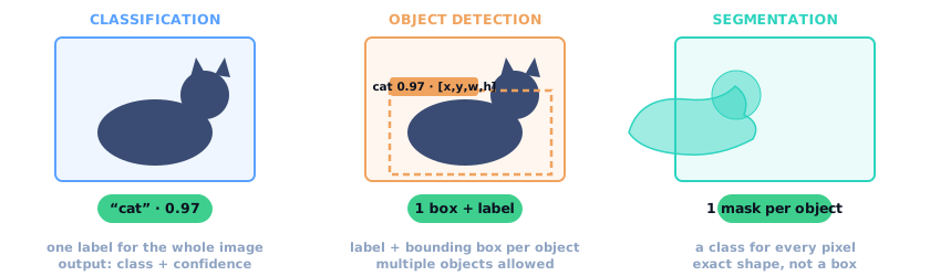
2Classification vs detection vs segmentation
Technical — outputs and losses
- Classification — output: one probability vector over classes. Loss: cross-entropy.
- Detection — output: N boxes, each
[x, y, w, h, class scores, objectness]. Loss: box regression (e.g., smooth-L1) + classification, plus the matching problem: which prediction counts for which object? (Solved by IoU matching → §6.) - Segmentation — output: per-pixel class map (semantic) or per-object masks (instance). Loss: pixel-wise cross-entropy / Dice. Architectures: encoder–decoder (U-Net style) that upsamples back to full resolution.
Common misconception
“Detection is just classification applied to patches.” Sliding-window classification exists but is hopelessly slow (thousands of crops per image) and redundant. Modern detectors predict all boxes in one or two passes (§4–5).
Knowledge check
A warehouse robot must grasp items — it needs exact object contours for the gripper. Which task, and why is a bounding box insufficient? Answer: (instance) segmentation. Boxes overlap for adjacent/tilted objects and don’t describe shape; a gripper needs the mask to plan contact points.
3CNN backbones & feature extraction
Technical
The backbone is the convolutional trunk (ResNet, CSPDarknet, EfficientNet…) that maps the input image to feature maps. It is exactly the Stage 2 §9 architecture minus the classifier head. Key idea: as depth grows, spatial resolution shrinks while each location summarizes a larger region — features become semantic (“this area contains fur and whiskers”) rather than geometric (“a diagonal edge here”).
- Feature pyramid — detectors usually consume several scales of the backbone (e.g., strides 8, 16, 32): fine maps for small objects, coarse maps for large ones (FPN, Lin et al. 2017).
- Receptive field — a detection head cell must “see” enough image to recognize its object; deep backbones provide this for free (Stage 2 §8).
- The detector head sits on top; the backbone is usually initialized from ImageNet pretraining (§9).
Knowledge check
Why do detectors need multi-scale feature maps instead of only the final one? Answer: the final map’s cells correspond to large image regions — small objects (a distant person, 10×20 px) collapse below resolvable detail there. Coarse layers handle big objects; fine layers handle small ones; a pyramid lets one model do both.
4YOLO — one-stage detection
Intuition
YOLO (“You Only Look Once”) divides the image into a grid — say 13×13 — and makes every cell answer simultaneously: “does an object sit centered on me? what class? where exactly does its box start and end relative to me?” All answers come out in one pass, like one giant classification over boxes. That is why it’s fast enough for video.
Technical — the mechanism
- Backbone produces the grid; each cell predicts B boxes + objectness (probability that a box contains any object) + class scores.
- Box coordinates are predicted relative to the cell (offsets + sizes) — easier to learn than absolute pixels, and each cell only proposes objects centered on it.
- One combined loss: localization (box regression) + objectness (binary) + classification — trained end-to-end.
- Consequences: extremely fast (single pass), global context (the whole image is seen when predicting each box) — but historically weaker on small/clumped objects than two-stage methods.
- Modern variants (v3–v8+, anchor-free designs, better heads) refine this recipe; the grid-in-one-pass idea is constant.
Common misconception
“YOLO’s name means it’s a gimmick.” It encodes the actual contribution: one look (single network evaluation) instead of thousands of window classifications or two-stage proposals.
Knowledge check
13×13 grid, 3 boxes per cell, 80 classes. How many raw box predictions per image? Answer: 13 × 13 × 3 = 507 boxes, each with 4 coords + 1 objectness + 80 class scores. Most are discarded by confidence thresholding and NMS (§7) before anything reaches the user.
5Faster R-CNN — two-stage detection
Intuition
Faster R-CNN splits the job. Stage 1 (RPN — Region Proposal Network) scans feature maps and proposes ~2,000 boxes that might contain anything. Stage 2 takes each proposed region, crops/aligns it from the feature maps, and classifies + refines it with full attention. Slow but thorough — a quality-over-speed trade.
Technical — RoI pooling in one sentence
Proposed boxes have arbitrary sizes, but stage 2 needs fixed-length vectors: RoI pooling crops each region out of the shared feature map and re-pools it to a fixed grid (e.g., 7×7) — so one classifier head handles all regions. Anchors: predefined box shapes/scales at each location that the RPN refines rather than predicting raw boxes from scratch. Simplification: modern variants replace anchors with learned predictions and improve the pooling (RoIAlign); the two-stage principle stands.
Knowledge check
You need real-time detection on a drone (30 FPS on small compute) vs the best possible mAP for an offline medical-image study. Which family for each, and why? Answer: drone → one-stage (YOLO family): latency budget dominates, single pass. Offline study → two-stage: per-region refinement buys accuracy when compute-per-image isn’t the constraint.
6Bounding boxes & IoU — worked by hand
Technical — the definition
A box is [x, y, w, h] or corner form [x1, y1, x2, y2]. Two boxes match
by Intersection over Union:
IoU(A, B) = area(A ∩ B) / area(A ∪ B) ∈ [0, 1]
1.0 = identical boxes; 0 = disjoint. Convention: a detection is a true positive at threshold t (commonly 0.5) if it overlaps its ground-truth object with IoU ≥ t, correct class, and no other prediction claimed that object first.
Compute it yourself — the four rules
- Intersection width =
min(x2A, x2B) − max(x1A, x1B); clamp negatives to 0. - Same for height.
- Intersection = w × h.
- Union = areaA + areaB − intersection. Divide.
Try: A = [0,0,10,10], B = [0,0,10,10] → IoU = 1. A = [0,0,10,10], B = [5,0,15,10] → inter 50, union 150 → 0.333. If B fully contains A, IoU = areaA / areaB.
Common misconception
“IoU 0.5 means 50% accurate localization.” It means the overlap occupies half the union — a box can miss half the object and still pass at t = 0.5. Strict applications (aerial imagery, crowded scenes) evaluate at 0.75 or 0.9.
Knowledge check
Prediction [0,0,100,100] for ground truth [0,0,100,50]. IoU? Does it pass at t = 0.5? Answer: inter = 100×50 = 5000; union = 10000 + 5000 − 5000 = 10000; IoU = 0.5 → passes exactly at t = 0.5 (boundary convention matters — usually ≥ counts). At t = 0.75 it fails.
7Non-maximum suppression — worked
Intuition
Detectors over-predict on purpose: many cells fire on the same object. NMS keeps the best-scoring box per object and deletes overlapping duplicates — keeping the summit, removing the foothills.
Technical — the algorithm
- Discard boxes with confidence below a threshold.
- Sort remaining by score, descending.
- Take the top box → keep it.
- Remove every remaining box with IoU > threshold (typically 0.5) against it.
- Repeat with the next-highest survivor until done.
Worked trace
Boxes (all same class): A score 0.90, B 0.80, C 0.85 — where C is nearly identical to A (IoU(A, C) = 1.0) and IoU(A, B) = 0.14. Threshold: score ≥ 0.3, IoU > 0.5.
- Sort: A (0.90), C (0.85), B (0.80).
- Keep A. Compare C: IoU 1.0 > 0.5 → suppress C. Compare B: IoU 0.14 ≤ 0.5 → keep.
- Next survivor: B → keep. Done.
Result: {A, B}. Duplicates die; genuinely different objects (or a person next to the cat) survive because their IoU is low.
Common misconception
“NMS works across classes.” Standard NMS is per-class — a ‘cat’ box and a ‘dog’ box at the same spot both survive (sometimes desired: occluding objects). Class-agnostic NMS exists for cases like “any vehicle.” Know which one your detector uses.
Knowledge check
Two people standing close together: NMS keeps only one box. Name two remedies. Answer: lower the NMS IoU threshold (e.g., 0.3) so heavily-overlapping-but-distinct boxes both survive; or use soft-NMS (down-weight instead of hard-remove) / class-agnostic settings tuned for crowds. Crowd-specific detectors (e.g., RepLoss-style) go further.
8Precision, recall & mean Average Precision
Intuition
Stage 1 §6 defined precision (“when I alarm, am I right?”) and recall (“of all real cases, how many did I catch?”). Detection reuses them, with IoU matching defining what a “hit” is. Because results depend on the confidence threshold, we sweep it: each threshold gives one (precision, recall) point — the curve traced is the Precision–Recall curve, and its area is average precision (AP).
Technical — the ladder from AP to mAP
- Match predictions to ground truth: sort by confidence; a prediction is TP if IoU ≥ t with an unclaimed GT of the same class; otherwise FP. (Each GT can be claimed once — duplicates are FPs.)
- AP at threshold t, per class = area under the precision–recall curve for that class (interpolated so the curve is monotonically non-increasing).
- mAP@t = mean of AP over all classes at threshold t. (PASCAL VOC used t = 0.5.)
- COCO mAP@[.5:.95] = mean of mAP over t = 0.50, 0.55, …, 0.95 — rewards precise localization, not just “found something.”
Related COCO metrics: APsmall / APmedium / APlarge (object-size slices) and AR (average recall at fixed detections per image). Report the exact metric name — “mAP 0.4” means nothing without the protocol.
Common misconception
“mAP is the mean of AP over images.” It is the mean over classes (then, for COCO, over IoU thresholds too). Per-image averaging is a different, nonstandard number.
Knowledge check
Model A: mAP@0.5 = 0.45, mAP@0.75 = 0.10. Model B: mAP@0.5 = 0.40, mAP@0.75 = 0.28. Which for a measuring application that needs tight boxes? Answer: B — its precision survives stricter thresholds; A “finds” objects but locates them loosely. This is exactly what mAP@[.5:.95] exposes.
9Transfer learning for detection
Technical
- Initialize the backbone from image-classification pretraining (COCO/ImageNet); replace the head with your class count.
- Fine-tune: heads first (higher LR), backbone at lower LR; unfreeze more if data allows. Detection needs more data than classification to fine-tune well — boxes are information-richer but scarcer annotations.
- Domain gap matters more than raw size: aerial/medical/industrial imagery may need full fine-tuning or domain-specific pretraining (Stage 2 §10 decision rule applies).
- Established toolchains:
torchvision.models.detection(Faster R-CNN, RetinaNet), MMDetection, Ultralytics YOLO — all ship pretrained checkpoints.
Knowledge check
Your fine-tuned detector excels on large objects, fails on small ones. Two concrete levers? Answer: train/evaluate with higher-resolution inputs (small objects gain pixels), and use multi-scale feature pyramids / assign small objects to finer pyramid levels; more small-object training examples (augmentation: scale-down copies, tiling) also helps.
10Grad-CAM: where the model looked
Intuition
Grad-CAM asks the gradients one question: “for this class’s score, how much did each last-layer feature map care about each spatial location?” Weight the maps by those importances, sum, rectify — you get a coarse heatmap of the image regions responsible for the prediction.
Technical — the recipe
- Forward pass; capture activations Ak of the last conv layer and the score yc for class c.
- Backward from yc; the gradient of yc w.r.t. each map is averaged spatially → weight αk.
- Class heatmap: ReLU( Σk αk Ak ), resize to image size.
LcGrad-CAM = ReLU( Σk αkc Ak ), αkc = (1/Z) Σi Σj ∂yc/∂Akij
Uses: debugging (model looking at watermark → dataset bias), failure analysis (§11), sanity-checking transfer learning. Limits: coarse (last-conv resolution), shows correlation with the prediction, not causal correctness; a good heatmap does not prove the model generalizes.
Knowledge check
Your pneumonia classifier scores well, but Grad-CAM highlights the chest-X-ray’s text label corner. What does this suggest, and what is the fix? Answer: shortcut learning — the model reads hospital/metadata burned into pixels instead of pathology. Fix: audit the dataset for leakage (crop the corner, balance sources across splits, retrain), not the model.
11Evaluation, failure analysis & dataset leakage
Technical — a failure-analysis loop
- Slice the metrics: mAP per class, per object size, per lighting/scene condition. Aggregate mAP hides everything.
- Read the confusion: which classes merge? (motorbike ↔ bicycle → fine-grained features missing or annotation inconsistency.)
- Inspect error types: localization-right/class-wrong; class-right/box-loose (fails at high IoU); duplicates (NMS mis-tuned); missed small objects.
- Grad-CAM a sample of errors — is the model looking at the object, the context, or a watermark?
- Fix at the dataset level first: more/better annotations of the failing slice usually beats architecture tweaks.
Common misconception — leakage, vision edition
“Leakage is a tabular-data problem.” Vision leaks too: near-duplicate photos across splits (same shoot, burst frames), video frames split randomly (adjacent frames are near-identical), all images from one hospital/source in train and another only in test, labels visible in pixels (§10’s X-ray case). Fix: split by source/scene/patient, dedupe by embedding similarity.
Knowledge check
Validation mAP drops 20 points after you re-annotate the test set with tighter boxes. Explain. Answer: evaluation got stricter (higher-quality boxes → matches require better localization); nothing about the model changed. Also check it isn’t the reverse: old boxes may have been lenient, inflating past scores. Metric comparability requires frozen annotation protocol — re-baseline both models under the new annotation.
12Quiz
Attempt each before expanding.
Q1 — IoU(A, B) with A=[0,0,10,10], B=[5,5,15,15]?
Intersection [5,5,10,10] → 25; union 100+100−25 = 175 → IoU ≈ 0.143. (§6)
Q2 — Why does YOLO need NMS even though each cell predicts few boxes?
Neighboring cells and multiple anchors all fire on one large object → many overlapping high-confidence predictions; NMS keeps one per object. (§4, §7)
Q3 — A prediction has IoU 0.7 with a GT already claimed by a higher-confidence prediction. TP or FP?
FP — each GT is claimed once; later overlapping predictions are duplicates. (§8)
Q4 — What does COCO mAP@[.5:.95] add over mAP@0.5?
It averages mAP over ten IoU thresholds — rewarding precise localization, exposing models that find objects but draw loose boxes. (§8)
Q5 — Grad-CAM highlights background. Two possible causes?
Shortcut/bias features in the dataset (watermarks, context correlation) or a genuinely context-driven prediction (legitimate but brittle). Either way: audit data before touching the model. (§10, §11)
Q6 — Why can’t you randomly split video frames into train/test?
Adjacent frames are near-identical → test frames leak via their neighbors in train; scores reflect memorized scenes. Split by video/scene. (§11)
13Exercise — IoU and NMS from scratch
Implementation challenge
Implement IoU and NMS in NumPy, verify the §6/§7 hand numbers, then cross-check against
torchvision.ops.nms. These two functions are interview staples and you will reuse
them in every detection project.
# iou_nms_exercise.py — pip install numpy torch torchvision
import numpy as np

def iou(a, b):
    """a, b: [x1, y1, x2, y2] → float in [0, 1]."""
    ix1, iy1 = max(a[0], b[0]), max(a[1], b[1])
    ix2, iy2 = min(a[2], b[2]), min(a[3], b[3])
    iw, ih = max(ix2 - ix1, 0), max(iy2 - iy1, 0)   # clamp: disjoint → 0
    inter = iw * ih
    area_a = (a[2]-a[0]) * (a[3]-a[1])
    area_b = (b[2]-b[0]) * (b[3]-b[1])
    return inter / (area_a + area_b - inter)

def nms(boxes, scores, iou_thr=0.5):
    """boxes: (N, 4), scores: (N,) → kept indices, highest score first."""
    order = np.argsort(scores)[::-1]
    keep = []
    while order.size:
        i = order[0]; keep.append(i)
        rest = order[1:]
        suppress = np.array([iou(boxes[i], boxes[j]) > iou_thr for j in rest])
        order = rest[~suppress]
    return keep

# --- Test 1: §6 hand example -------------------------------------------------
A = [100,100,200,200]; B = [150,150,250,250]
assert abs(iou(A, B) - 2500/17500) < 1e-9
assert iou(A, A) == 1.0
assert iou([0,0,10,10], [20,20,30,30]) == 0.0  # disjoint, no crash

# --- Test 2: §7 NMS trace -----------------------------------------------------
boxes  = np.array([A, B, A], dtype=float)          # C == A on purpose
scores = np.array([0.90, 0.80, 0.85])              # A, B, C
assert nms(boxes, scores, 0.5) == [0, 1]          # keep A, B; suppress C

# --- Cross-check against torchvision -----------------------------------------
import torch
from torchvision.ops import nms as tv_nms
ref = tv_nms(torch.tensor(boxes), torch.tensor(scores), 0.5)
assert nms(boxes, scores, 0.5) == ref.tolist()
Deliverables: (1) all asserts pass; (2) one-paragraph answer: why does NMS sort before comparing, and what breaks if you compare in input order? Stretch: implement soft-NMS (decay overlapping scores instead of removing: s ← s·(1 − IoU)) and construct a two-object case where hard NMS loses an object but soft-NMS keeps it; vectorize your IoU over all pairs (broadcasting) and benchmark vs the loop version.
14References
- Redmon et al. — “You Only Look Once: Unified, Real-Time Object Detection,” CVPR 2016, arXiv:1506.02640: arxiv.org/abs/1506.02640
- Ren et al. — “Faster R-CNN: Towards Real-Time Object Detection with Region Proposal Networks,” arXiv:1506.01497: arxiv.org/abs/1506.01497
- Lin et al. — “Feature Pyramid Networks for Object Detection,” arXiv:1612.03144: arxiv.org/abs/1612.03144
- Lin et al. — “Microsoft COCO: Common Objects in Context” (metrics definition), arXiv:1405.0312: arxiv.org/abs/1405.0312 · official eval protocol
- Selvaraju et al. — “Grad-CAM: Visual Explanations from Deep Networks via Gradient-based Localization,” ICCV 2017, arXiv:1610.02391: arxiv.org/abs/1610.02391
- torchvision — detection models & ops: pytorch.org/vision · torchvision.ops.nms
Primary papers and official docs, verified at writing time. Metric definitions follow the COCO protocol; where this sheet simplifies (anchors, RoIAlign, soft-NMS variants), the simplification is labeled in place.
Progress checklist
Ticks persist in this browser only (localStorage).
Provenance: structured sheet from Batch 3 of the AI Learning Lab project — a personal study resource, not a claim of expertise. Verify specifics against the references before use in graded work.
Last reviewed: not yet — set this date after your first full pass.
Transformers and LLMs · sheet 2 of 2 in this chapter
LLM Fundamentals
1What is an LLM?
Intuition
An LLM is a next-token predictor of enormous scale. Trained to continue text on a vast corpus, it is forced to absorb grammar, facts, style, reasoning patterns — anything that helps predict the next token better. All impressive behaviors (translation, coding, Q&A) are downstream of that single objective.
Technical — the three claims in the name
- Language — models text sequences; everything else is representation learned en route.
- Model — a transformer (decoder-only, mostly) with billions of parameters — the numbers training adjusts (Stage 2: training changes weights; inference uses them).
- Large — scale across three axes at once: parameters, data (tokens), compute. GPT-3 (2020): 175B parameters, ~300B training tokens (published figures). Scaling laws (Kaplan 2020; Chinchilla/Hoffmann 2022) quantify how loss falls predictably as all three grow — Chinchilla’s rule of thumb: ~20 training tokens per parameter for compute-optimal pretraining.
What it is not: a database (facts live lossily in weights), a search engine (no lookup without retrieval — see Chapter 4), or a logic engine (probabilistic, sampled outputs).
Common misconception
“An LLM knows things.” Mechanically, it computes the next-token distribution given context — knowledge exists only as statistical tendencies encoded in weights, retrieved by continuing text. That framing explains both its fluency and its failure modes (§9).
Knowledge check
A 7B-parameter model trained on 14T tokens — over- or under-trained relative to the Chinchilla rule of thumb? Answer: ~2,000 tokens/param vs ~20 recommended → heavily over-trained (data-rich, inference-optimized): smaller models trained longer. This is the modern “small-model-overtrained-for-deployment” recipe.
2The full pipeline: text in → response out
Two details the diagram hides
- Streaming: the loop emits each token as soon as it’s sampled — that’s why chat UIs type word-by-word; the pipeline runs once per token, not once per answer.
- Stop conditions: generation ends on a stop token (e.g., EOS) or a max-token budget. The model has no built-in notion of “finished my point” beyond learned EOS behavior.
Knowledge check
An answer of 200 tokens required how many forward passes (ignoring KV-cache optimizations)? Answer: 200 — one per generated token. (With KV caching, each pass is cheaper, but the count stays one per token.)
3Tokenization & why it matters beyond the model
Technical — the product view
- Cost & limits are token-denominated: API pricing, context limits, and rate limits all count tokens, not words. English averages roughly ~4 characters/token (varies by domain and tokenizer).
- Tokenization is per-model: the same text has different token counts under GPT-2 vs Llama-3 tokenizers. Always measure with the actual tokenizer — never guess from words.
- Failure modes follow the vocabulary: rare languages fragment into many tokens (longer, costlier, sometimes weaker performance), arithmetic and letter-counting suffer because numbers and words aren’t digit-letter sequences to the model (Stage 2 §1).
- Round-trip is guaranteed —
decode(encode(x)) == x— but word boundaries are not: “chatGPT” might be two tokens, “GPT” another single one.
Knowledge check
A product must keep a conversation under a 4,096-token window. Why is estimating with “average words × 1.3” dangerous? Answer: token-to-word ratios vary hugely by language, domain (code fragments heavily), and tokenizer; a long non-English or code-heavy history can blow the budget while the estimate says it fits. Count with the real tokenizer at runtime.
4Embeddings: static vs contextual
Technical — two different vectors called “embedding”
- Token embedding (static, input): a fixed learned vector per vocabulary entry — row lookup (Stage 2 §2). The same vector for “bank” everywhere.
- Contextual representation (per position, per layer): after attention mixes information across tokens, each position’s vector is context-specific: “bank” near “river” vs “money” becomes different vectors inside the network. This is the real mechanism behind “understanding”: geometry shaped by context.
Consequences: (1) meaning is compositional — sentence representations differ from any bag of word vectors; (2) this is why the same model can do sentiment, translation, and code — contexts induce the needed geometry; (3) embedding models for retrieval (Chapter 4) are encoder-only systems trained so that semantically similar texts land close together — a different training objective on the same broad idea.
Common misconception
“Embeddings are the model’s dictionary of meanings.” The static table is more like an address book — the meaning-making happens in the contextual geometry built by attention and MLPs across layers.
Knowledge check
Why can’t the static token embedding alone distinguish “bank” in the two sentences? Which component does? Answer: the lookup is context-free by construction. Self-attention: the “bank” token’s query pulls in information from surrounding tokens (“river”/“loan”), shifting its contextual vector — from layer to layer the representation disambiguates.
5Logits → probabilities → sampling
Technical — the math
pi = exp(zi / T) / Σj exp(zj / T)
- Logits z — raw, unnormalized scores, one per vocabulary entry.
- Temperature T — divides logits before softmax. T = 1: the model’s honest distribution. T < 1 sharpens (more deterministic); T > 1 flattens (more random). T → 0 equals argmax.
- Top-k — zero out all but the k highest-probability tokens, renormalize, sample.
- Top-p (nucleus) — keep the smallest set of tokens whose cumulative probability ≥ p, renormalize, sample. Adapts the cut: 2 candidates when the model is confident, 50 when unsure.
Worked — the same logits at two temperatures
Logits: [2.0, 1.0, 0.5].
T = 1: softmax([2, 1, 0.5]) = e²/(e²+e¹+e^0.5) = 7.389/11.756 → [0.628, 0.231, 0.140].
T = 0.5: logits double → softmax([4, 2, 1]) = 54.60/64.71 → [0.844, 0.114, 0.042] — sharper. T = 2 would flatten toward uniform.
Top-p = 0.9 at T = 1: sorted cumulative: 0.628 → 0.859 → 0.999. The smallest set with cumsum ≥ 0.9 is {tokens 1, 2} → keep two, renormalize to [0.731, 0.269], sample. The long tail never gets sampled.
Common misconception
“Temperature adds randomness to a fixed answer.” It changes the shape of the probability distribution before sampling; there is no fixed answer underneath. Also: temperature doesn’t make the model smarter or dumber — it trades coherence vs variety at the margins.
Knowledge check
Why does top-p usually behave better than fixed top-k across domains? Answer: top-k cuts a constant number of options whether the distribution is confident (k=50 includes junk) or flat (k=50 amputates good candidates); top-p keeps a quality mass, adapting the count to the model’s certainty.
6Pretraining: what, why, how much
Technical
- Objective: next-token prediction over trillions of web/book/code tokens — self-supervised (labels are the data, Stage 1 §2; mechanics Stage 2 §9).
- What it buys: grammar, world knowledge, style transfer, in-context pattern completion — compressed statistically into weights. No labels, no tasks, just continuation.
- Result — a base model: a brilliant autocomplete with no notion of being an assistant. Prompt “The capital of France is” → likely completes fine; prompt with a question and it may continue with more questions, because that’s what pages of Q&A look like.
- Scale figures (published): GPT-3: 175B params / ~300B tokens. Chinchilla: 70B / ~1.4T tokens — compute-optimal, and it beat the 10× larger Gopher. Modern models train far beyond Chinchilla-optimal for deployment efficiency (§1’s check question).
Connect to your repo: TinyShakespeare pretraining is exactly this loop at 1/10⁶ scale — loss ln(65)≈4.17 → ~1.5, samples emerging from noise.
Common misconception
“Pretraining teaches the model to follow instructions.” It teaches prediction. Instruction following is instilled afterwards (§7) — that’s why chatting with a raw base model feels alien.
Knowledge check
Why does a base model complete “How do I make bread?” with more questions instead of an answer? Answer: on the training distribution, text resembling that prompt (forums, FAQ pages) frequently continues with further questions/other users’ text. The model reproduces the document-style continuation — it has no “assistant” role until tuned into one.
7Fine-tuning, instruction tuning, preference optimization
Technical — stage 3 without the folklore
- RLHF: humans rank answer pairs → train a reward model to predict preferences → optimize the policy (the LLM) against that reward with RL (PPO), tethered to the SFT model by a KL penalty so it doesn’t drift into reward-hacking gibberish.
- DPO: a closed-form alternative — skip the reward model, optimize the policy directly on preference pairs with a classification-style loss. Simpler, stable, widely used in open models. Simplification: DPO and PPO optimize related but not identical objectives; each has failure modes (reward hacking vs off-policy limits).
- Parameter-efficient variants: LoRA freezes weights, trains small low-rank adapters — a fraction of the memory, mergeable afterwards (your Phase 2 plan; Stage 2 §10 is the same principle for CNN backbones).
Common misconception
“Fine-tuning teaches facts.” It reliably teaches form and behavior; new facts are better injected via retrieval (Chapter 4) — fine-tuned facts are lossy, unattributable, and prone to spaghetti with pretraining knowledge.
Knowledge check
Your chatbot must answer only from a legal corpus with citations. Fine-tune or RAG — and why not fine-tune the facts in? Answer: RAG: inject documents at query time, get citations and updates by re-indexing, control access per user. Fine-tuning facts: no provenance, stale on any corpus update, and it cannot guarantee coverage of “everything in the corpus.” Fine-tuning is still useful — for tone/format/refusals — layered on top of RAG.
8The context window
Technical — three honest caveats about “1M context”
- Effective use ≠ nominal length: models recall best at the ends; long middles are under-used (“lost in the middle” effect). Marketing window ≠ reliable working memory.
- Cost scales with length: attention is quadratic in context per pass; you pay in latency and money for every token, every step.
- No persistence: between requests, only what your app re-sends exists. “Memory” features are engineering (store & re-inject), not weight changes.
Knowledge check
Your RAG app retrieves 10 chunks × 400 tokens each and answers start to degrade. Diagnose and fix? Answer: likely context crowding — relevant chunks diluted by mediocre ones (and mid-window placement). Fix: retrieve fewer/better chunks (reranking — Chapter 4), put best chunks first/last, compress history, and measure answer quality vs chunk count instead of assuming more context is better.
9Hallucinations & limitations
Intuition
Because it was never trained to be true — only to continue plausibly. When the training distribution says “questions like this are usually followed by confident answers,” the model produces a confident answer-shaped string, whether or not the fact lives in its weights. Hallucination is the objective functioning as designed, in an unintended niche.
Technical — the main failure families
| Failure | Mechanism | Mitigation |
|---|---|---|
| Fabricated facts/citations | plausible continuation over absent knowledge | RAG + citations; ask for “unknown” option; verify critical outputs |
| Stale knowledge | frozen weights, cutoff date | retrieval; tools/APIs for live data |
| Arithmetic / counting | tokens aren’t numbers; no built-in calculator | tool use (code execution); decompose steps |
| Overconfidence in tone | SFT amplifies confident style; calibration suffers | prompt for uncertainty; sample multiple answers; calibrate judges |
| Prompt injection | untrusted text in context can redirect behavior | treat retrieved/user text as untrusted; validate tool outputs (Chapter 4) |
Positioning: none of these are “bugs” in one implementation — they are properties of the paradigm. Engineering (retrieval, tools, evals — Chapters 4–5) is how products survive them.
Common misconception
“Bigger models stop hallucinating.” Scale reduces some errors but introduces new plausible- sounding ones (more convincing fabrications). Grounding (retrieval/tools) and evaluation, not scale alone, bend the curve.
Knowledge check
Why does asking the same hallucinating model “are you sure?” often flip the answer? What does that reveal? Answer: each turn is a fresh conditional distribution — the new context (question + its answer) shifts probabilities; there is no internal fact-checker being consulted, just re-sampling conditioned on doubt. Reveals: no persistent self-model of its own certainty → design for verification, not interrogation.
10Quantization & inference efficiency
Technical — store weights in fewer bits
- Post-training quantization (PTQ): convert trained weights to INT8/INT4 with careful scaling (methods: GPTQ, AWQ, llama.cpp’s k-quants). Small quality dips, huge memory wins; usually negligible for chat use.
- QLoRA: quantize the frozen base to 4-bit, train LoRA adapters on top — fine-tuning on consumer GPUs (your Phase 2 compute plan).
- KV cache: past keys/values stored per layer to avoid recomputing them each token — memory grows with context length; this (not weights) often dominates long-context serving.
- Other levers (one-line each): batching many requests, speculative decoding (a small draft model proposes, the big model verifies), FlashAttention kernels.
Common misconception
“Quantization shrinks the model’s knowledge.” It compresses the numerical representation of the same weights — knowledge is mostly intact; what degrades (slightly) is precision of the computations. Confusing storage precision with model size in parameters is a category error.
Knowledge check
You must serve a 13B model on one 16 GB GPU with 8K context. Where does memory go, and what’s the plan? Answer: weights FP16 = 26 GB — doesn’t fit → INT4 (~6.5–7 GB); KV cache at 8K context for batch 1 is typically several GB (layers × heads × dims × 2 × 2 bytes × tokens) — budget it; remaining headroom for activations. Plan: 4-bit weights + paged/quantized KV cache + modest batch. (Exact KV numbers depend on architecture — compute from config, don’t guess.)
11Quiz
Attempt each before expanding.
Q1 — Logits [3, 1] at T=1: probabilities? (mental math, e³≈20.1, e¹≈2.72)
softmax = [20.1/22.8, 2.72/22.8] ≈ [0.88, 0.12]. At T=2 (logits halved → [1.5, 0.5]): e^1.5≈4.48 → [4.48/7.20, 2.72/7.20] ≈ [0.62, 0.38] — flatter. (§5)
Q2 — Base vs instruct model: what changed, and at which stage?
Same architecture; weights changed in SFT (+ often stage 3) to follow instructions — objective and data changed, not the transformer itself. (§6–7)
Q3 — Why is RAG better than fine-tuning for “answers only from our 2,000-page manual”?
Retrieval guarantees the exact text enters the context at query time, gives provenance/citations, updates by re-indexing, allows per-user access control. Fine-tuned facts are lossy, unstaleable, unattributable. (§7, §9)
Q4 — Two different “embedding” meanings in one LLM — name both.
Static token-embedding table (input lookup) and contextual per-position representations after attention/MLP layers. (§4)
Q5 — A 8B model at FP16 doesn’t fit your 12 GB GPU. Two independent levers?
Quantize weights (INT8 ≈ 8 GB or INT4 ≈ 4–5 GB) and/or shrink KV-cache footprint (shorter context, quantized/paged cache). Both compose. (§10)
Q6 — Your manager: “the model learned our docs from last week’s chat.” Correct them precisely.
No weight updates happened; the chat only filled the context window. Without your app re-sending that text, the model has zero memory of it. (§8)
12Exercise — sampling from scratch
Implementation challenge
Implement temperature softmax, top-k, and top-p in NumPy, assert the §5 worked numbers, then
swap your implementation into the GPT repo’s generate() and compare samples.
# sampling_exercise.py — pip install numpy torch
import numpy as np

def softmax_temp(logits, T=1.0):
    z = np.asarray(logits, dtype=float) / max(T, 1e-8)
    z -= z.max()                                  # stability
    e = np.exp(z)
    return e / e.sum()

def top_k_filter(logits, k):
    out = np.array(logits, dtype=float)
    thresh = np.sort(out)[-k]                     # k-th largest value
    out[out < thresh] = -np.inf
    return out

def top_p_filter(logits, p):
    probs = softmax_temp(logits)
    order = np.argsort(probs)[::-1]
    cum = np.cumsum(probs[order])
    keep = order[cum - probs[order] < p]          # smallest set with mass ≥ p
    out = np.full_like(probs, -np.inf)
    out[keep] = logits[keep]
    return out

def sample(logits, T=1.0, top_k=None, top_p=None, rng=None):
    z = np.array(logits, dtype=float)
    if top_k:  z = top_k_filter(z, top_k)
    if top_p:  z = top_p_filter(z, top_p)
    probs = softmax_temp(z, T)                    # -inf → exp 0 automatically
    assert abs(probs.sum() - 1) < 1e-6
    return int(rng.choice(len(probs), p=probs)) if rng else int(np.random.choice(len(probs), p=probs))

# --- Tests: §5 worked numbers ------------------------------------------------
logits = [2.0, 1.0, 0.5]
assert np.allclose(softmax_temp(logits, 1.0), [0.628, 0.231, 0.140], atol=1e-3)
assert np.allclose(softmax_temp(logits, 0.5), [0.844, 0.114, 0.042], atol=1e-3)

# top-p = 0.9 at T=1 keeps exactly 2 tokens
f = top_p_filter(logits, 0.9)
assert np.isfinite(f).sum() == 2, f

# top-k = 1 → deterministic argmax
rng = np.random.default_rng(0)
picks = {sample(logits, T=1.0, top_k=1) for _ in range(20)}
assert picks == {0}

# cross-check softmax against torch
import torch
ref = torch.softmax(torch.tensor(logits) / 1.0, dim=-1).numpy()
assert np.allclose(softmax_temp(logits), ref, atol=1e-7)
Deliverables: (1) all asserts pass; (2) replace the temperature/top-k block in your
repo’s generate() with these functions (keep behavior identical — A/B a few prompts);
(3) stretch: implement min-p filtering (keep tokens with p ≥ min_p · p_max), which
newer stacks ship, and describe in one paragraph when it beats fixed top-k.
13References
- Brown et al. — “Language Models are Few-Shot Learners” (GPT-3, scale + in-context learning), arXiv:2005.14165: arxiv.org/abs/2005.14165
- Kaplan et al. — “Scaling Laws for Neural Language Models,” arXiv:2001.08361: arxiv.org/abs/2001.08361
- Hoffmann et al. — “Training Compute-Optimal Large Language Models” (Chinchilla), arXiv:2203.15556: arxiv.org/abs/2203.15556
- Ouyang et al. — “Training language models to follow instructions with human feedback” (InstructGPT / RLHF), arXiv:2203.02155: arxiv.org/abs/2203.02155
- Rafailov et al. — “Direct Preference Optimization” (DPO), arXiv:2305.18290: arxiv.org/abs/2305.18290
- Holtzman et al. — “The Curious Case of Neural Text Degeneration” (top-p / nucleus sampling), arXiv:1904.09751: arxiv.org/abs/1904.09751
- Dettmers et al. — “QLoRA: Efficient Finetuning of Quantized LLMs,” arXiv:2305.14314: arxiv.org/abs/2305.14314 · llama.cpp (PTQ in practice): github.com/ggerganov/llama.cpp
- Ji et al. — “Survey of Hallucination in Natural Language Generation,” arXiv:2202.03629: arxiv.org/abs/2202.03629
Primary papers, verified at writing time. Scale figures (GPT-3 175B/300B tokens, Chinchilla 70B/1.4T, ~20 tokens/param) are the papers’ published numbers; no benchmark scores are quoted on this sheet.
Progress checklist
Ticks persist in this browser only (localStorage).
Provenance: structured sheet from Batch 3 of the AI Learning Lab project — a personal study resource, not a claim of expertise. Verify specifics against the references before use in graded work.
Last reviewed: not yet — set this date after your first full pass.
The source material is preserved in full. Open the complete original HTML collection.