 [ BESMALA ]
AI Engineering · 2 study sheets
Batch 05
Move from model development to production, then examine evaluation and responsible AI.
AI Engineering and Deployment · sheet 1 of 2 in this chapter
AI Engineering: From Model to Production
1Experimentation vs AI engineering
Intuition
A trained model is a file that computes a function. A product is that file wrapped in everything that makes it reachable, safe, observable, and recoverable: an API, validation, containers, secrets, monitoring, rollback. The model is one box among many — and usually the smallest one.
Technical — what changes at the transition
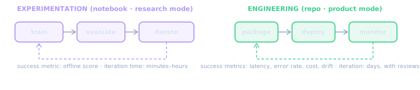
| Dimension | Notebook | Production |
|---|---|---|
| Inputs | clean local CSV | hostile, partial, adversarial requests |
| Failure mode | exception you read | 5xx alerts at 3 a.m., silent drift |
| Reproducibility | “ran fine yesterday” | pinned versions, images, artifacts |
| Change control | rerun the cell | CI → review → staged rollout → rollback |
| Owner of quality | you | tests + monitors + on-call process |
Connect to our repo: train.py + Colab is the left loop. This sheet builds the
right loop around rag.py / a model checkpoint.
Common misconception
“Deployment = calling model.predict() from Flask.” Serving is maybe 20% of the
surface. The other 80% — validation, packaging, secrets, observability, rollout, rollback — is
what distinguishes a demo from a system.
Knowledge check
Name three questions a reviewer should ask about a “94% accurate” model before it ships. Answer: any three of: 94% on what split, with what leakage controls? At what latency/cost per request? How does it fail on out-of-distribution inputs? How will drift be detected after launch? Can it be rolled back?
2Python project organization
Technical — a layout that scales
my-ai-service/
├── pyproject.toml          # dependencies + metadata (single source of truth)
├── Dockerfile              # built in CI, never by hand (§7)
├── src/service/
│   ├── main.py             # FastAPI app (§4) — thin, imports the rest
│   ├── inference.py        # load artifact, predict — pure, testable
│   ├── schemas.py          # Pydantic request/response models (§5)
│   └── settings.py         # env-var config, no hardcoded secrets (§8)
├── tests/
│   ├── test_api.py         # fast tests via TestClient (§11)
│   └── fixtures/           # tiny model copy for tests — never the 4 GB one
└── .github/workflows/ci.yml
- Importable package (
src/layout) — tests and server import the same code the notebook proved out; no copy-pasted preprocessing. - Notebooks are for exploration only — anything a service needs gets promoted into
src/with tests. Notebook code is a draft, not a dependency. - Config lives in settings.py reading env vars (§8); behavior changes without code edits.
Common misconception
“Structure is cosmetic.” Structure determines what can be tested: if preprocessing is inline in the endpoint, you cannot unit-test it; if config is hardcoded, every environment change is a code change and a redeploy.
Knowledge check
Your API imports preprocessing from notebooks/prep_v2.ipynb via a copied function.
What two risks does the §2 layout remove? Answer: (1) drift between the notebook version
and the served copy (train/serve skew — §6); (2) untestability — a copied function inside the
endpoint can’t be unit-tested in isolation. Both vanish when one imported, tested
inference.py is the single definition.
3Model serialization & loading
Technical — the formats
| Format | Best for | Risk |
|---|---|---|
| pickle / joblib | sklearn pipelines, quick local work | executes arbitrary code on load — never unpickle untrusted files; breaks across library versions |
| safetensors | LLM/transformer weights | safe (pure data, no code execution), fast mmap loads — the modern default for weights |
| ONNX | portable graphs across runtimes/languages | op-set coverage varies by exporter |
| native checkpoints | PyTorch .pt with config | pair weights with the config/processor files — weights alone are not a model |
Ship a bundle, not a file: weights + preprocessing artifacts (the fitted scaler! §6) + config + a version string. Versioned in object storage (S3 §10), referenced by exact path or hash — “latest” is how 3 a.m. incidents start.
artifact size = params × bytes/param — our GPT ≈ 10.8M × 4 B ≈ 43 MB (fp32) → ≈ 21 MB (fp16)
Common misconception
“Pickle is fine internally.” Internally still means: anyone with repo write access, any compromised dependency, any misconfigured bucket can plant a pickle that runs code on your servers at load time. Load-time code execution is a privilege you grant deliberately or not at all.
Knowledge check
Why does the preprocessing scaler belong in the versioned artifact next to the weights? Answer: serving must reproduce training-time transforms exactly (§6). If the scaler is refitted or lost, inputs are silently transformed differently — no crash, just quietly wrong predictions, which is the worst failure class.
4REST APIs & FastAPI
Technical — the minimal serving core
# main.py — the whole skeleton; sections below harden it
from fastapi import FastAPI
from pydantic import BaseModel, Field
from service.inference import Predictor

app = FastAPI(title="my-ai-service", version="1.2.0")
predictor = Predictor()          # loads the artifact bundle once, at startup

class PredictIn(BaseModel):
    text: str = Field(min_length=1, max_length=8000)

class PredictOut(BaseModel):
    label: str
    confidence: float

@app.get("/healthz")
def healthz():
    return {"status": "ok"}          # liveness: process is up

@app.get("/readyz")
def readyz():
    return {"ready": predictor.ready}  # readiness: model actually loaded

@app.post("/v1/predict", response_model=PredictOut)
def predict(body: PredictIn):
    return predictor.predict(body.text)
- REST in one line: resources at URLs, manipulated with methods (GET/POST/…),
JSON bodies, status codes as the contract. Version the path (
/v1/) so breaking changes get a new route, not angry clients. - FastAPI gives Pydantic validation (§5), automatic OpenAPI docs at
/docs, and dependency injection — the framework choice here because the learning curve is small and the guardrails are real. - Load the model once at startup (module scope or lifespan event) — reloading per request is the classic first-deploy performance bug.
Common misconception
“Async everywhere makes AI serving faster.” Model inference is CPU/GPU-bound, not I/O-bound:
def endpoints run in a threadpool and are fine; async def shines when
awaiting I/O (remote APIs, databases). Sprinkling await around a blocking
predict() gains nothing and can block the event loop.
Knowledge check
Why two health endpoints instead of one? Answer: liveness (“process running”) tells the orchestrator to restart a wedged container; readiness (“model loaded, warm”) tells the load balancer to route traffic. Collapsing them sends real traffic to containers that booted but haven’t loaded a 43 MB artifact yet.
5Request validation & error handling
{"text": null} and a 40 MB string. Then what?Technical — the hardening layers
- Schema validation (Pydantic) — types, lengths, ranges, required fields. Invalid requests fail before touching the model with 422 Unprocessable Entity and a precise error message. Free, declarative, self-documenting.
- Body-size and rate limits — at the gateway/proxy (§9), not just app code: reject absurd payloads and abusive clients cheaply.
- Timeouts everywhere — per-request server timeout, per-dependency timeouts. A slow downstream must degrade one endpoint, not hang the fleet.
- Correct status codes: 400/422 client error · 401/403 auth · 503 when the model
isn’t ready or is overloaded (lets load balancers route around you) · 500 for genuine bugs.
Never return 200 with
{"error": ...}— monitoring can’t see it (§12). - Fail with a contract:
{"error": {"code": "MODEL_OVERLOADED", "message":
      "retry after N"}}
— machine-readable errors are part of your API.
Common misconception
“Validation is UX nicety.” It’s a security and cost control: an unvalidated 10 MB input hits your tokenizer before anyone checks anything — you pay compute for hostile traffic. Validate at the boundary, cheaply, first.
Knowledge check
Your model returns a NumPy float32. FastAPI serializes it and errors on JSON encoding. Where
should the fix live, and why not in the route? Answer: in inference.py /
the response schema — convert to native Python float at the inference boundary (or
declare the Pydantic type and let it coerce). Routes should orchestrate, not patch types; fixing
it at the source keeps the function reusable and the schema honest.
6Inference pipelines & train/serve skew
Technical — the pipeline and its one law
request → validate → preprocess(exactly as training) → model → postprocess → response
Train/serve skew = any difference between the training-time and serving-time transformations. The classic killers:
- Recomputed statistics: serving refits the scaler per request/batch instead of loading the training-fitted one (§3’s artifact bundle exists to prevent this).
- Two implementations: notebook preprocessing pasted into the API and edited once (§2’s layout exists to prevent this).
- Version drift: serving upgrades a tokenizer/library that training used differently — pin and test both sides together.
- Distribution shift (real-world inputs moving — not a bug, a fact of life): monitored in the Evaluation sheet §10; skew is your bug, shift is time’s. Diagnose them separately.
Test it like you mean it: a golden-set test that feeds known inputs through the served endpoint and asserts predictions match the training-time outputs bit-for-bit (or within tolerance). This single test catches most skew classes automatically.
Knowledge check
Post-deploy accuracy drops with zero code changes. Name one skew cause and one shift cause, and say which you can fix in the next deploy. Answer: skew example: the scaler/tokenizer version in the serving image differs from training’s (fixable — pin, redeploy). Shift example: the population changed since the training window (not fixable by redeploy — retrain/monitor).
7Docker & containerization
Technical — the image is the environment
# Dockerfile — pin the base; small context; non-root; one job per container
FROM python:3.11-slim-bookworm

WORKDIR /app
COPY pyproject.toml ./
RUN pip install --no-cache-dir .          # deps layer cached between builds
COPY src/ ./src/

RUN useradd -m appuser && USER appuser     # never root in production
EXPOSE 8000
CMD ["uvicorn", "service.main:app", "--host", "0.0.0.0", "--port", "8000"]
- Why containers: the image bundles interpreter + libraries + code + system deps — the same bytes run on your laptop, CI, and the cloud. “Works on my machine” becomes “works on every machine, identically.”
- Layers & caching: each instruction is a cached layer; copying
pyproject.tomlbefore source means dependency installs cache while you iterate on code — minutes to seconds per build. - Hygiene:
.dockerignore(never ship.git/, datasets, local.env); pin base images (digest for real rigor); one process per container; the model artifact usually loads from S3 at startup (§9) rather than bloating the image — decide deliberately per size.
Common misconception
“Docker is a VM.” Containers share the host kernel and isolate processes/namespaces — they’re fast to start (seconds) and cheap to run, which is exactly what makes autoscaling (§9, §12) practical. VMs virtualize hardware; containers package a process.
Knowledge check
Your Docker build reinstalls all dependencies on every code change. What’s wrong with the layer order? Answer: source was copied before dependency installation — any source edit invalidates the install layer. Order: copy dependency manifest → install → copy source. (§7’s Dockerfile does exactly this.)
8Environment variables & secrets
Technical — 12-factor config
- Config = environment: the same image runs dev/staging/prod; only env vars change (Twelve-Factor App, config principle). Code never branches per environment — config does.
- Hierarchy of homes for secrets: local dev →
.envfile, git-ignored forever; cloud → a secrets manager or the platform’s secret store injected at task start; never in code, never in the image, never in git history (history is forever and public scanners crawl it). - Least privilege pairs with secrets: a secret only earns its keep with an IAM role that limits what it can touch (§10) — a leaked key for a read-only bucket is a bad afternoon; a leaked admin key is a breach.
- Rotation: treat secrets as perishable — rotation story exists on day one, not after an incident.
# settings.py — typed config, fail fast at boot, not at 3 a.m.
import os
MODEL_URI = os.environ["MODEL_URI"]            # crashes at startup if missing — good
LOG_LEVEL = os.environ.get("LOG_LEVEL", "INFO")
MAX_TEXT  = int(os.environ.get("MAX_TEXT", "8000"))
Common misconception
“Private repo, so keys in code are OK.” Private repos get shared, forked, cloned to laptops, and leaked via CI logs — and insider access isn’t threat-model-free. Secrets live in secret systems; that’s the whole job.
Knowledge check
A teammate commits an AWS key, then deletes the file in the next commit. Why is the key still burned? Answer: it remains in git history (anyone can check out the old commit), and it may already be mirrored in CI logs/forks. The response is rotate-and-revoke, not delete — and a pre-commit scanner so it doesn’t recur.
9The production architecture — one request’s journey
The request’s life, step by step
- Client sends
POST /v1/predictover TLS to the load balancer (the only public door — everything else lives in private subnets). - LB forwards to one healthy ECS task (readiness gate, §4).
- Pydantic validates the body — garbage dies here with 422, never reaching the model (§5).
inference.pypreprocesses with the training-fitted artifacts (§6).- Model (loaded once at startup from the S3 artifact bundle, §3) runs; NumPy types become JSON-safe native types.
- Structured log line ships to CloudWatch: request id, latency, prediction confidence (§12).
- Response returns; the task is immediately free for the next request. Concurrency and replicas — not a queue you hand-rolled — absorb the load (§12).
Why each box exists, in one line each: LB = one stable address + TLS + health-aware routing · ECS = run/replace/scale containers without babysitting servers · S3 = durable versioned artifacts decoupled from images · ECR = the versioned image that produced these running containers · IAM = the reason a leaked app bug can’t delete your bucket · CloudWatch = the flight recorder and the alarm bell · RDS = the app’s relational state, private like the tasks.
Knowledge check
Why does the model artifact live in S3 rather than baked into the image? Give two reasons and one counter-case for baking it in. Answer: (1) image and model version independently — new model, zero rebuild; (2) large artifacts bloat images, slowing pull/start and autoscale. Counter-case: small models (< few MB) baked in give fully self-contained, faster cold starts and simpler rollouts — a legitimate choice when sizes allow.
10The AWS service map
Technical — one row per service, tied to the diagram
| Service | What it is | Role in this deployment |
|---|---|---|
| IAM | identity & permission system | the task’s role can read the artifact bucket and write logs — nothing else. Every arrow in §9 crosses an IAM check. |
| S3 | versioned object storage | model bundles (s3://bucket/model/v1.2.0/), datasets, backups; cheap, durable, publicly sealed. |
| ECR | private Docker registry | stores the built image per version; ECS pulls from it. Image registry ↔ artifact store are separate on purpose (§9 check). |
| ECS (+ Fargate) | container orchestration | runs N copies of the container, replaces dead ones, scales on demand. Fargate = serverless compute for tasks (no EC2 babysitting). |
| EC2 | raw virtual machines | the underlying option — you manage the OS, sizing, and fleets. Use when you need GPU nodes or deep control; Fargate otherwise. |
| VPC | your private network | public subnet: only the LB. Private subnets: tasks and RDS with no inbound internet. Network boundaries are a security layer, not red tape. |
| RDS | managed relational DB | the app’s Postgres/MySQL — users, records, or pgvector embeddings; managed backups, patches, failover. |
| CloudWatch | logs, metrics, alarms | where every request’s log line lands; where p95/5xx/CPU alarms page a human (§12). |
| EKS | managed Kubernetes | the same architecture when the org standardizes on k8s: richer orchestration, steeper price in complexity. ECS-first unless k8s is already a team skill. |
Simplification: each service has dozens of features; this table is the 10% that carries 90% of AI-serving deployments. The concepts (network tiers, least privilege, versioned artifacts, telemetry) transfer to GCP/Azure verbatim.
Common misconception
“EKS is the upgrade from ECS.” It’s a sidestep, not an upgrade: EKS buys the k8s ecosystem and costs an ops tax. Teams migrate for organizational reasons (portability, existing tooling), not because ECS “isn’t enough” for serving a model.
Knowledge check
Your task’s IAM role accidentally includes s3:* on the whole bucket. Why does §9
call this an incident-in-waiting even with perfect code? Answer: the role is part of the
attack surface — any future bug (SSRF, dependency compromise, injected instruction — AI Agents §9)
inherits those powers. Least privilege caps the blast radius of code you haven’t written yet.
11CI/CD & testing
Technical — the pipeline stages
# .github/workflows/ci.yml (essentials)
jobs:
  test:
    steps:
      - run: pip install -e .[dev] && pytest -q        # unit + API tests
  build-push:
    needs: test
    steps:
      - run: docker build -t $ECR/repo:$GIT_SHA .       # sha-tagged, never "latest"
      - run: docker push $ECR/repo:$GIT_SHA
  deploy-staging:
    needs: build-push
    steps:
      - run: aws ecs update-service --task-def new ...  # then smoke tests hit /healthz
- Test pyramid for ML services: unit (preprocessing, schemas — fast, no model), integration (API + tiny fixture model end-to-end via TestClient), golden-set (served predictions match training-time outputs — the skew test, §6), smoke (the deployed staging endpoint answers, healthy, in budget).
- CI = Continuous Integration: every push runs the tests. CD = Continuous Delivery/Deployment: the green build becomes a running version automatically — through staging at minimum, canary in production (§13).
- Tag images with the git SHA — the running version and the code version become the same thing, which makes rollbacks a tag flip, not an archaeology dig.
Common misconception
“ML systems can’t be tested — the model is nondeterministic.” The code is perfectly testable (schemas, preprocessing, error paths); the model is testable on fixed fixtures with tolerance; the service is testable contract-first. Non-determinism is a reason for golden-set tolerances, not an excuse to skip CI.
Knowledge check
CI is green but staging’s p95 tripled after deploy. Which test layer should have caught it, and why didn’t unit tests? Answer: the smoke/performance gate on staging — unit tests run on a laptop without realistic payload sizes or resource limits (and possibly a debug-mode server). Latency is a deployment-environment property: gate it where it lives.
12Logging, monitoring, latency & scalability
Technical — the observability trio
- Logs — structured JSON per request:
{request_id, route, latency_ms,
      status, confidence}
. Structured beats string logs because it’s queryable; request IDs stitch a request’s journey across boxes. - Metrics — aggregated numbers over time: request rate, error rate, latency percentiles, CPU/memory. Percentiles, not averages: an average of 150 ms is compatible with 5% of users waiting 2 s — and those users complain the loudest. p95/p99 are the contract.
- Alarms — on symptoms users feel (p95 over budget, 5xx rate), not on every cause (single CPU spikes). Every alarm must have an owner and a runbook, or it trains everyone to ignore alarms.
Worked — a latency budget that adds up
Target: p95 ≤ 300 ms for /v1/predict.
| Stage | p50 | p95 budget |
|---|---|---|
| network + LB | 30 ms | 60 ms |
| validation | 1 ms | 2 ms |
| preprocess (tokenize) | 12 ms | 25 ms |
| model forward | 90 ms | 140 ms |
| postprocess + serialize | 6 ms | 12 ms |
| total | ≈139 ms | ≈239 ms ✓ headroom |
The model owns the big share — optimize there only after the tail is honest: profile, batch small requests (trade a few ms of waiting for 3–5× throughput), or quantize (LLM Fundamentals §10: same weights, fewer bytes → faster memory-bound steps).
Scalability — the two levers
capacity ≈ replicas × (1 / p50_service_time) · 4 replicas × (1/0.14 s) ≈ 28 req/s
- Vertical — bigger machines (more CPU/RAM/GPU). Quick, capped, and wastes money at 3 a.m. traffic lows.
- Horizontal — more replicas, autoscaled on CPU or request rate; stateless services (ours is — all state is in S3/RDS, §9) scale horizontally for free. This is the default.
- The batching trade: grouping requests raises throughput but adds queue wait — tune max batch size and max wait against the p95 budget, not vibes.
Common misconception
“We monitor the model’s accuracy in production.” You monitor proxies until labels arrive — inputs, outputs, latency, error rate — and drift detection (Evaluation sheet §10) bridges the gap. Accuracy needs ground truth; production rarely labels itself promptly.
Knowledge check
p50 is 140 ms but p99 is 2.1 s. Name three classic tail-latency causes. Answer: any three of: cold starts (new replica loading the artifact before ready — §4’s readiness gate), GC/pauses or noisy neighbors, unbounded queueing under burst (batch wait configured too long), a slow downstream dependency without timeouts (§5), oversized payloads hitting validation last.
13Model versioning & deployment strategies
Technical — the registry + the rollout patterns
- Model registry (MLflow-style): every trained model registered with its version, metrics, data hash, and artifact URI. Promotion is a decision on record: candidate → staging → production. “Which model is live?” must be a query, not a memory.
- Rollback is a feature you build before you need it: keep the previous task definition one command away; re-point to the prior S3 artifact. Rehearse it in staging.
Common misconception
“Better offline metrics → just ship it to everyone.” Offline gains evaporate under serving conditions (§6), and the first minutes of a bad rollout cost more than every canary delay ever did. The Evaluation sheet’s discipline plus a canary is the whole method.
Knowledge check
Your canary at 5% shows p95 +80 ms and error rate 0.3%→0.9%. What happens next, mechanically and in order? Answer: the metrics gate trips → automatic rollback (shift 100% back to v1.2; the canary task definition is terminated) → the incident note links the canary’s request IDs and logs (§12) → diagnosis offline → fix → new canary. Widen-only-while-healthy is the entire policy.
14Quiz
Attempt each before expanding.
Q1 — Why load the model at startup instead of per request?
Load cost (tens of MB–GB, deserialize, warm caches) would be paid on every request — p99 would be dominated by cold loads. Startup-once + readiness gating means only new replicas pay it. (§4)
Q2 — A request with a 2 MB body arrives. Name the two cheapest places it dies.
The gateway/body-size limit at the proxy (rejected before your fleet spends anything), then Pydantic max_length validation (422). Both are boundary checks that precede any model compute. (§5)
Q3 — Serving refits the StandardScaler on each batch. Which section’s failure is this, and why don’t errors appear?
Train/serve skew (§6). No errors because the transform still “works” — it just normalizes with per-batch statistics instead of training statistics; predictions are silently wrong, which is why the golden-set test exists.
Q4 — Why is the load balancer the only component in a public subnet?
Minimize the attack surface: exactly one TLS-terminating door is reachable from the internet; tasks and RDS accept traffic only from inside the VPC. Network boundaries back up IAM (§10).
Q5 — Capacity math: p50 service time 140 ms, 6 replicas. Rough req/s?
6 × (1/0.14) ≈ 43 req/s — before concurrency within a replica, which raises it further. Use the number for floor-planning, then load-test. (§12)
Q6 — Blue/green vs canary: which needs spare capacity, and which caps user exposure first?
Blue/green needs ~2× capacity during cutover but switches atomically; canary needs little extra capacity and caps exposure (5%) from the first minute. Choose by risk profile and budget. (§13)
15Exercise — a testable, containerized API
Implementation challenge
Build the smallest honest version of §4–§11: a FastAPI service with a trivial “model,” validation, health/readiness, error contract — and a pytest suite that runs it all offline. Then containerize it and write the Dockerfile layer-order fix from §7’s check question.
# pip install fastapi uvicorn pytest httpx      (no GPU, no downloads)
# app.py
from fastapi import FastAPI
from pydantic import BaseModel, Field

app = FastAPI(title="mini-ai-service")

class PredictIn(BaseModel):
    text: str = Field(min_length=1, max_length=200)

class PredictOut(BaseModel):
    label: str
    confidence: float

_state = {"ready": False}

@app.on_event("startup")
def load_model():
    # pretend this loads a 43 MB artifact — the point is: once, at startup
    _state["model"] = lambda t: ("positive", min(0.99, 0.5 + 0.01 * len(t)))
    _state["ready"] = True

@app.get("/healthz")
def healthz(): return {"status": "ok"}

@app.get("/readyz")
def readyz():
    return {"ready": _state["ready"]} if _state["ready"] else ({"ready": False}, 503)

@app.post("/v1/predict", response_model=PredictOut)
def predict(body: PredictIn):
    label, conf = _state["model"](body.text)
    return PredictOut(label=label, confidence=conf)

# test_api.py — the whole pyramid, miniature: schema, contract, skew-gate
from fastapi.testclient import TestClient
from app import app

client = TestClient(app)

def test_ready_gates_traffic():
    assert client.get("/readyz").status_code == 200   # startup ran

def test_validation_rejects_garbage():
    r = client.post("/v1/predict", json={"text": ""})         # too short
    assert r.status_code == 422
    r = client.post("/v1/predict", json={"wrong_field": "x"})  # bad schema
    assert r.status_code == 422

def test_happy_path_contract():
    r = client.post("/v1/predict", json={"text": "great model"})
    assert r.status_code == 200
    body = r.json()
    assert set(body) == {"label", "confidence"}   # the response contract
    assert 0.0 <= body["confidence"] <= 1.0

def test_deterministic_same_input():
    # miniature golden-set: identical input → identical output (§6 discipline)
    a = client.post("/v1/predict", json={"text": "skew test"}).json()
    b = client.post("/v1/predict", json={"text": "skew test"}).json()
    assert a == b
Dockerfile task: write it with the wrong layer order first (copy everything,
then install), measure rebuild time after a one-character code change; then reorder per §7 and
re-measure. Deliverables: all four tests pass (pytest -q); the 422s come back
with readable error bodies; the two rebuild timings written down with the why.
Stretch: add a /v1/predict-batch endpoint with a max-size limit and one test
proving oversize batches get 422 — you’ve now built §5 twice, which is the point.
16References
- FastAPI — official documentation (validation, async, deployment): fastapi.tiangolo.com
- Docker — packaging/container concepts and Dockerfile reference: docs.docker.com
- The Twelve-Factor App — config, backing services, disposability: 12factor.net
- AWS — documentation for IAM, S3, ECS, VPC, ECR, RDS, CloudWatch, EKS
- Google SRE Book — monitoring, alerting, SLOs (free online): sre.google
- MLflow — model registry and tracking: mlflow.org
- Hugging Face — safetensors: huggingface.co/docs/safetensors · ONNX: onnx.ai
- Burkov — Machine Learning Engineering (the discipline this sheet compresses): mlebook.com
Official docs and primary sources, verified at writing time. No invented internal benchmarks: the latency table in §12 is a worked example budget, labeled as such — measure your own.
Progress checklist
Ticks persist in this browser only (localStorage).
Provenance: structured sheet from Batch 5 of the AI Learning Lab project — a personal study resource, not a claim of expertise. Companion: AI Evaluation and Responsible AI (below). Verify specifics against the references before use in graded work.
Last reviewed: not yet — set this date after your first full pass.
Research and Evaluation · sheet 2 of 2 in this chapter
AI Evaluation and Responsible AI
1Why accuracy alone is insufficient
Technical — three structural reasons
- Base rates: with 0.5% prevalence, “always negative” scores 99.5% while catching nothing. Accuracy conflates class frequency with model skill.
- Asymmetric costs: a missed tumor and a false alarm both subtract one from accuracy — and are not remotely the same event. One number cannot encode a cost ratio of 100:1.
- Aggregation hides slices: 90% overall can hide a 30-point subgroup gap (§7). Any single number is an average over distributions you haven’t examined.
What replaces it: a metric set chosen from the problem (§2), evaluated per slice (§5, §7), with calibration checked when probabilities drive decisions (§6), and a decision threshold justified in writing (§2’s worked cost).
Common misconception
“Evaluation is a step at the end.” It’s the frame around the whole project: metrics and thresholds are decided before modeling (or the results quietly bend toward whatever the model happens to be good at). The template in §11 enforces that order.
Knowledge check
A teammate reports “95% accuracy, ship it.” What three follow-up questions do you ask before any discussion of the number itself? Answer: any three of: prevalence of the positive class? per-slice breakdown (§7)? what threshold, and chosen how (§2)? precision/recall trade at that threshold? evaluated on what split with what leakage controls (Stage 1 §3)? compared against what baseline (§11 template)?
2Choosing metrics from the problem — the cost argument, worked
Technical — expected cost of a threshold
E[cost](t) = FN(t)·CFN + FP(t)·CFP
For each candidate threshold t, count the confusion-matrix cells and price them. Pick t that minimizes expected cost. This is the entire method — and it must be done with numbers written down.
Worked — cancer screening, 1,000 patients, 1% prevalence
10 true positives exist. Costs: CFN = 10,000 (missed case), CFP = 100 (follow-up test). The model scores 1,000 patients; two thresholds on the same model:
| Threshold | TP | FN | FP | TN | Expected cost |
|---|---|---|---|---|---|
| t = 0.3 | 9 | 1 | 50 | 940 | 1×10,000 + 50×100 = 15,000 |
| t = 0.7 | 7 | 3 | 10 | 980 | 3×10,000 + 10×100 = 31,000 |
The lower threshold wins by 2× despite five times the false alarms — because one missed case costs 100 follow-ups. Sensitivity to the ratio: at CFN=CFP the higher threshold would win. The threshold is a property of the cost table, not of the model — which is why it’s chosen with stakeholders, in writing, before deployment.
Common misconception
“Threshold 0.5 is the default because it’s optimal.” It’s optimal only under symmetric costs and calibrated probabilities. For imbalanced-cost problems the default is silently costing money or lives — §6 shows probabilities may not even mean what 0.5 implies.
Knowledge check
Same screening model, but the follow-up test becomes painful and expensive: CFP = 5,000. Re-price both thresholds — which wins now? Answer: t=0.3: 10,000 + 250,000 = 260,000; t=0.7: 30,000 + 50,000 = 80,000 → t=0.7 wins. The identical model flipped its best threshold because the world changed — metrics live in context.
3Classification & regression evaluation, extended
Technical — the additions
- PR-AUC vs ROC-AUC under imbalance: ROC-AUC’s false-positive rate is computed against the huge negative class, flattering weak models on rare positives; PR-AUC stays honest about the class you care about (Saito & Rehmsmeier, 2015). Rule: rare positives → report PR-AUC.
- Macro vs micro averaging: macro = unweighted mean of per-class metrics (every class counts equally); micro = pooled counts (frequent classes dominate). Worked: class A (990 examples): P=R=0.99 → F1≈0.99; class B (10 examples): P=0.5, R=0.3 → F1 = 2·0.15/0.8 = 0.375. Macro F1 = (0.99+0.375)/2 ≈ 0.68 — the rare class drags it down, honestly. Micro ≈ 0.985 — nearly invisible. Report macro when rare classes matter.
- Regression beyond a single number: MAE/RMSE/R² (Stage 1 §6) plus the residual plot — errors vs prediction, vs each feature, over time. Patterns in residuals (funnels, curvature, seasonality) are diagnoses a scalar can’t give: heteroscedasticity, missing interaction, drift.
Common misconception
“R² = 0.9 means the model is good.” R² is relative to predicting the mean — on easy data it’s trivially high; on the transformed target (logs, diffs) it isn’t comparable to the original scale. Always pair R² with a units-bearing error (MAE/RMSE) and the residual plot.
Knowledge check
Your 3-class model reports micro-F1 0.96, macro-F1 0.61. What happened, and which classes do you investigate? Answer: a frequent class is nearly perfect while one or more rare classes perform poorly; the pooled average drowns them. Investigate the rare classes’ precision/recall individually (error analysis, §5) and consider data collection or reweighting.
4Robustness & distribution shift
Technical — the shift taxonomy
| Type | What changes | Example | Detect via |
|---|---|---|---|
| Covariate shift | P(X) — inputs | new camera sensor; new dialect in text | input-distribution monitoring (§10) |
| Concept drift | P(Y|X) — the mapping | “fraud patterns” evolve against you | performance decay once labels arrive |
| Label shift | P(Y) — class mix | seasonal disease prevalence | prediction-distribution monitoring |
- Robustness testing before deployment: evaluate on deliberately perturbed inputs — image noise/brightness/crops; text paraphrases and typos; missing values. A model that collapses under mild perturbation memorized textures, not features (CV sheet’s Grad-CAM cross-check, Stage 3).
- Time-based splits as the honest rehearsal for deployment: train on month 1–11, test on month 12. Random splits let the model peek at the future (Stage 1 §3’s temporal leakage).
- OOD inputs: decide the behavior by design — detect-and-abstain beats confident nonsense (LLM Fundamentals §9’s “I don’t know” is the same principle).
Common misconception
“More training data fixes shift.” It fixes coverage of the training distribution. Shift is about the future belonging to a distribution you can’t fully sample — the remedies are monitoring, robustness testing, and retraining loops (§10 below).
Knowledge check
Your classifier held 94% for a year; input distributions look stable; accuracy is now 88%. Which shift type fits, and what additional evidence confirms it? Answer: concept drift — P(Y|X) moved while P(X) didn’t. Confirm with labeled outcomes (support tickets, audits, delayed ground truth) showing the same inputs now map to different labels; prediction-distribution monitoring alone won’t show it.
5Error analysis: the loop
Technical — the categorization that matters
- Label noise — the “truth” was wrong; fix the dataset (and the annotation process), not the model.
- Genuine ambiguity — humans disagree too; define policy (collect more labels, add an “uncertain” class, or accept and document).
- Capability gap — consistent, systematic errors the model should get: the real improvement target. Sub-categorize by feature (lighting, dialect, rare class).
- Leakage/eval bugs — errors that appear when you fix the split (Stage 1 §3): sometimes the “errors” were a broken test all along.
The rule: no architecture change until 50 errors are read and categorized. Most “we need a bigger model” conclusions dissolve into “we need cleaner labels for slice X.”
Knowledge check
Error analysis finds 60% of errors are mislabeled ground truth. Why is retraining the wrong first move? Answer: training against noisy targets optimizes toward noise; the model’s apparent errors partly measure the annotators. Fix: re-annotate the affected slices (measure inter-annotator agreement), correct the set, then retrain — and fix the labeling process that produced the noise.
6Calibration — when 0.8 should mean 80%
Intuition
A classifier can be accurate and dishonest: it may be right 90% of the time while claiming 99% every time. Calibration is the honesty property — among cases predicted at 0.8, is the real frequency ≈ 0.8? Deep networks are famously overconfident (Guo et al., 2017).
Technical — the two measures
ECE = Σbins (nb/N) · |accuracyb − confidenceb| · Brier = (1/N) Σ (pi − yi)2
ECE (expected calibration error): bin predictions by confidence, weigh each bin’s |accuracy − confidence| gap by its size. Brier: mean squared error of probabilities — a proper scoring rule that rewards both discrimination and honesty.
Worked — ECE on 300 predictions, 3 bins
| Confidence bin | n | avg confidence | accuracy | |gap| | weighted gap |
|---|---|---|---|---|---|
| [0.00, 0.33) | 100 | 0.20 | 0.25 | 0.05 | (100/300)·0.05 = 0.0167 |
| [0.33, 0.66) | 50 | 0.50 | 0.40 | 0.10 | (50/300)·0.10 = 0.0167 |
| [0.66, 1.00] | 150 | 0.80 | 0.70 | 0.10 | (150/300)·0.10 = 0.0500 |
ECE = 0.0167 + 0.0167 + 0.0500 ≈ 0.083 — the model is systematically overconfident (claims 0.8, delivers 0.7).
Brier, mini-version: predictions (0.9, y=1), (0.2, y=0), (0.6, y=1) → (0.1)² + (0.2)² + (0.4)² = 0.01+0.04+0.16 → mean = 0.07.
The fix: temperature scaling — one temperature T fitted on validation data, applied to logits before softmax (LLM Fundamentals §5’s T, reused post-hoc). Cheap, preserves ranking (accuracy unchanged), restores meaning to the probabilities — which is exactly what §2’s thresholding assumes.
Common misconception
“Calibration fixes accuracy.” It changes no predictions under argmax — only the confidence numbers. Its value is downstream: thresholds (§2), risk scores presented to humans, and abstention rules all assume probabilities mean what they say.
Knowledge check
Why must temperature T be fitted on validation data rather than training data? Answer: on training data the model is (near-)fitted already — its confidence/accuracy relationship there doesn’t represent deployment; T fitted on train undercorrects. Validation (or a held-out calibration set) is where honest confidence gaps live.
7Bias & subgroup evaluation
Worked — the average that hides the gap
1,000 users: 900 majority, 100 minority.
| Group | n | accuracy | correct |
|---|---|---|---|
| majority | 900 | 93% | 837 |
| minority | 100 | 63% | 63 |
| overall | 1,000 | 90% | 900 |
“90% accuracy” is arithmetic truth and an ethical lie by omission: a 30-point service gap against the smaller group, fully invisible without the slice. Subgroup evaluation is not an optional add-on; it is the evaluation.
Technical — where bias enters, and the metric families
- Entry points: unrepresentative data collection (who got sampled?), label bias (historical decisions as ground truth), proxy features (postcode standing in for race, name for gender), and measurement differences across groups.
- Common metric families (each encodes a value judgment): demographic parity (similar positive rates across groups), equal opportunity (similar true-positive rates), equalized odds (similar TPR and FPR). These can be mutually unsatisfiable with different base rates — choosing one is a policy decision with stakeholders, not a coding task.
- The operational habit: report every headline metric per group, plus the gaps; audit the errors per group (who gets false positives? who gets missed?). Fairness work starts as measurement, and measurement starts with the slices.
Simplification: “fairness” has no single formal definition — the field maps which definitions conflict and when (fairmlbook.org). Anyone selling “the fairness metric” is selling one value judgment as neutral.
Common misconception
“Removing the sensitive attribute removes the bias.” Proxies resurrect it — correlated features carry much of the signal. Removal changes the audit trail, not the behavior; only subgroup evaluation reveals what remains.
Knowledge check
A hiring model drops gender and passes overall accuracy parity across regions. Name two checks that could still surface bias. Answer: (1) per-group error decomposition — TPR/FPR gaps (equalized-odds view) that accuracy parity hides; (2) proxy audit — measure how much removed-attribute signal survives in correlated features (predict the attribute from the remaining features; high predictability = the proxy lives). Then stakeholder decisions on which metric family to prioritize.
8Data privacy & security
Technical — the working rules
- Data minimization: collect and retain only what the task needs. Every extra field is liability with a schema. Define retention periods and enforce deletion.
- Anonymization vs pseudonymization: anonymization removes re-identification paths (hard — re-identification research keeps proving “anonymized” sets re-identifiable); pseudonymization replaces identifiers with keys you hold (useful, still personal data under GDPR-style regulation — treat it accordingly).
- Models memorize: trained models can leak training data (membership-inference and extraction attacks). Consequences: don’t train on data you can’t defend having; consider privacy techniques (differential privacy, PII scrubbing) for sensitive corpora; LLM-specific surfaces (injection, exfiltration via tools) are AI Agents §9.
- Baseline hygiene: encryption in transit and at rest, strict access control (§10’s IAM), audit logs of who accessed what — the boring 90% of “AI security.”
Common misconception
“We deleted the names, so it’s anonymous.” Quasi-identifiers (birth date + postcode + gender) uniquely identify most people in practice. Anonymization is a property to be tested against re-identification, not a checkbox after dropping a column.
Knowledge check
A stakeholder wants to fine-tune on support tickets containing customer emails “for personalization.” Design the minimal responsible pipeline. Answer: (1) purpose limitation — is personalization worth personal data? (2) PII scrubbing/regex+NER redaction before training; (3) access control + retention on the ticket store; (4) evaluate extraction risk (can the model be prompted to emit a redacted-incorrect email? test it); (5) document all of it. If the answer to (1) is “not really,” the rest is moot — minimization first.
9Reproducibility
Technical — the five pins
- Code version — the exact commit (git SHA), including config files.
- Data version — dataset hash or versioned snapshot (DVC-style); data changes are the silent killer of “same code, different number.”
- Environment — pinned dependencies (lockfile) or the container digest (§7); “pip install torch” is not a specification.
- Seeds & determinism — set seeds for python/numpy/framework; honest limits: GPU nondeterminism (atomic adds in some kernels) can persist; bit-exactness may require deterministic-algorithm flags and still isn’t guaranteed across hardware. Aim for statistically equivalent, and say which you achieved.
- Experiment tracking — log params, metrics, artifacts per run (MLflow/W&B) so every result links to its five pins automatically. The query “which run produced the shipped model?” must be one click.
Common misconception
“Reproducibility is academic pedantry.” It’s operational: debugging a deployed model starts with reproducing its behavior; audits and compliance ask for provenance; and “we can’t rerun it” means every future improvement competes against a number no one can verify.
Knowledge check
Same code, same seed, two runs — val loss differs by 0.02. Most likely explanation, and what would you log to distinguish candidates? Answer: most likely nondeterministic GPU kernels (or data-loader worker ordering) rather than “seeds didn’t work.” Log: exact container digest, GPU type/count, framework version, dataloader worker config, and whether deterministic flags were set — the pins of §9 turn mystery into diagnosis.
10Model limitations & monitoring
Technical — the production evaluation loop
- Input monitoring (no labels needed): feature/input distributions vs training reference — drift scores (e.g., PSI-style comparisons per feature, KS tests) alert when the world leaves the training distribution (§4’s covariate shift detector).
- Output monitoring: prediction distributions and confidence histograms — a slow slide toward all-one-class, or calibration sagging, is visible before any label arrives.
- Performance monitoring (labels when they arrive): delayed ground truth (chargebacks, diagnoses, human review samples) evaluated on rolling windows, per slice (§7). §12’s service metrics tell you the system is healthy; this tells you the model still is.
- The retraining decision is a policy: define triggers (drift threshold, performance floor, calendar) and the full path: retrain → this sheet’s evaluation on fresh data → §13’s canary. No ad-hoc “someone noticed.”
- Know the ceiling: document limitations explicitly — known OOD failure modes, groups with thin data, abstention behavior. The limitations section of §11’s template is a deliverable, not a confession.
Knowledge check
Inputs are stable, outputs are stable, but delayed labels show accuracy sliding. What is this, and which lever exists before retraining? Answer: concept drift (§4) — the mapping changed beneath stable marginals. Pre-retraining levers: recalibrate (§6, if confidence shifted), adjust thresholds per §2’s new cost reality, and route the degraded slice to human review while the retrain loop runs.
11The experiment-report template
Experiment report — [model / change name] · v[n] · date [YYYY-MM-DD]
- Hypothesis & change — what was tried, why, and what would falsify it.
- Success criteria (set BEFORE running) — primary metric, target value, evaluation split; the decision threshold and its cost rationale (§2); what result would mean “abandon.”
- Data — source, version/hash (§9), split method with leakage controls (Stage 1 §3), known gaps in coverage.
- Baselines — previous model and the trivial baseline (majority class / heuristic); improvement is only meaningful relative to both.
- Results — headline metric with uncertainty (across folds/seeds, §9); full confusion matrix or residual diagnostics (§3); per-slice table (§7) with gaps; calibration summary (§6) if probabilities are used.
- Error analysis — the 50-error read (§5): category counts, examples, what was fixed.
- Robustness — perturbation results, OOD behavior, time-split performance (§4).
- Limitations & risks — known failure modes, thin-data groups, privacy notes (§8).
- Decision & next step — ship / iterate / abandon, with the owner and date. The template ends in a decision, or it wasn’t an evaluation.
Common misconception
“Reports are bureaucracy.” The template’s real function is pre-registration: success criteria written before results prevent the human tendency to redefine success afterward. It is the scientific method wearing a project hat.
Knowledge check
Which template section, if written last instead of first, loses its entire purpose? Answer: success criteria (item 2). Written after results, thresholds and targets bend to fit what the model achieved — the pre-registration is the anti-rationalization device.
12The evaluation checklist (per release)
Twelve ticks is the honest bar. Ship with fewer only as a written, explicit exception.
13Quiz
Attempt each before expanding.
Q1 — Why does ROC-AUC flatter weak models under extreme imbalance, where PR-AUC stays honest?
FPR divides by the enormous negative count, so thousands of false positives barely move it; precision (in PR) divides by your own positive predictions, so every false alarm costs visibly. (§3)
Q2 — Model claims 0.9 on a bucket that’s right 0.75 of the time. Over- or under-confident, and which fix preserves accuracy exactly?
Overconfident (gap 0.15 → contributes to ECE). Temperature scaling — it monotonicly rescales confidences without changing the argmax ranking, so accuracy is untouched. (§6)
Q3 — Inputs and outputs look stable, delayed labels show decay. Diagnosis and the pre-retrain levers?
Concept drift. Levers: recalibrate, re-threshold per the current cost table, human-review the degraded slice — then retrain. (§4, §10)
Q4 — Why is “we removed gender” insufficient evidence of fairness?
Proxies preserve much of the signal, and accuracy parity hides TPR/FPR gaps. You need per-group error decomposition and a proxy-predictability audit. (§7)
Q5 — ECE check: bin n=200, conf 0.7, acc 0.6; overall N=400. This bin’s weighted gap?
|0.7−0.6| = 0.10 × (200/400) = 0.05. Same recipe as §6’s table — the size-weighting is what makes ECE reflect how many users experience each gap.
Q6 — Which template item is pre-registration, and what failure mode does it prevent?
Success criteria written before results (§11 item 2). Prevents post-hoc redefinition of success — the human tendency to move the goalposts to wherever the model landed.
14Exercise — calibration & subgroups from scratch
Implementation challenge
NumPy only: implement ECE (fixed-width bins), Brier score, and per-group accuracy gaps; assert every worked number from §6 and §7; then demonstrate that temperature scaling fixes confidence without touching accuracy.
# eval_exercise.py — pip install numpy
import numpy as np

def ece(probs, y_true, n_bins=10):
    """Expected Calibration Error, fixed-width bins (§6)."""
    probs, y_true = np.asarray(probs, float), np.asarray(y_true, int)
    bins = np.minimum((probs * n_bins).astype(int), n_bins - 1)
    total = 0.0
    for b in range(n_bins):
        m = bins == b
        if not m.any(): continue
        conf, acc = probs[m].mean(), y_true[m].mean()
        total += m.mean() * abs(conf - acc)     # size-weighted gap
    return total

def brier(probs, y_true):
    return float(np.mean((np.asarray(probs, float) - np.asarray(y_true, int)) ** 2))

# --- Test 1: §6's three-bin ECE table, reconstructed exactly -----------------
probs = np.array([0.20]*100 + [0.50]*50 + [0.80]*150)
y     = np.array([0]*25 + [1]*75  + [0]*30 + [1]*20  + [0]*45 + [1]*105)
assert abs(ece(probs, y, n_bins=3) - 0.0833) < 1e-3, ece(probs, y, n_bins=3)

# --- Test 2: §6's Brier mini-example -----------------------------------------
assert abs(brier([0.9, 0.2, 0.6], [1, 0, 1]) - 0.07) < 1e-9

# --- Test 3: §7's subgroup gap ------------------------------------------------
acc_majority, n_majority = 0.93, 900
acc_minority, n_minority = 0.63, 100
overall = (acc_majority*n_majority + acc_minority*n_minority) / (n_majority + n_minority)
assert abs(overall - 0.90) < 1e-9            # the average that hides 30 pts
assert acc_majority - acc_minority == 0.30   # the gap the slice reveals

# --- Test 4: temperature scaling fixes confidence, not accuracy ---------------
logits  = np.log(np.clip(probs, 1e-9, 1) / (1 - np.clip(probs, 1e-9, 1)))
def softmax(z, T=1.0):
    z = z / T; z -= z.max(axis=-1, keepdims=True)
    e = np.exp(z); return e / e.sum(axis=-1, keepdims=True)
before = (probs > 0.5).astype(int)
after  = (softmax(logits.reshape(-1, 1), T=2.0).ravel() > 0.5).astype(int)
assert (before == after).all()               # argmax unchanged → accuracy preserved
assert ece(softmax(logits.reshape(-1, 1), T=2.0).ravel(), y, 3) < ece(probs, y, 3)
# ↑ on this synthetic set, softening moves confidence toward the observed rates

print("all asserts passed — §6 and §7 verified in code")
Deliverables: (1) all asserts pass; (2) one paragraph: why the last assert compares ECE before/after while the previous asserts accuracy equality — what does that pair of checks encode about §6’s claim? Stretch: fit T on a held-out split to minimize ECE (1-D search) rather than hand-picking 2.0, and report the fitted T; then add macro- vs micro-F1 (§3’s worked numbers) to the same file.
15References
- Guo, Pleiss, Sun, Weinberger — “On Calibration of Modern Neural Networks,” ICML 2017, arXiv:1706.04599: arxiv.org/abs/1706.04599
- Saito & Rehmsmeier — “The Precision-Recall Plot Is More Informative than the ROC Plot When Evaluating Binary Classifiers on Imbalanced Datasets,” PLOS ONE 2015: journals.plos.org
- Barocas, Hardt, Narayanan — Fairness and Machine Learning (fairmlbook.org): fairmlbook.org
- NIST — AI Risk Management Framework (AI RMF 1.0): nist.gov
- scikit-learn — Model evaluation guide (metrics, calibration): scikit-learn.org
- Evidently — open-source drift & data-quality monitoring: docs.evidentlyai.com
- Chen et al. — Reliable Machine Learning (O’Reilly, 2022): oreilly.com
Primary papers, official frameworks, and official docs, verified at writing time. The worked numbers (ECE 0.083, Brier 0.07, the 90%-hides-30-points example) are constructed teaching examples, clearly labeled — not published benchmark results.
Progress checklist
Ticks persist in this browser only (localStorage).
Provenance: structured sheet from Batch 5 of the AI Learning Lab project — a personal study resource, not a claim of expertise. Companion: AI Engineering: From Model to Production (above). Verify specifics against the references before use in graded work.
Last reviewed: not yet — set this date after your first full pass.
The source material is preserved in full. Open the complete original HTML collection.